Fit Mixed-Effects Spline Regression

This example shows how to fit a mixed-effects linear spline model.

Load the sample data.

load('mespline.mat');

This is simulated data.

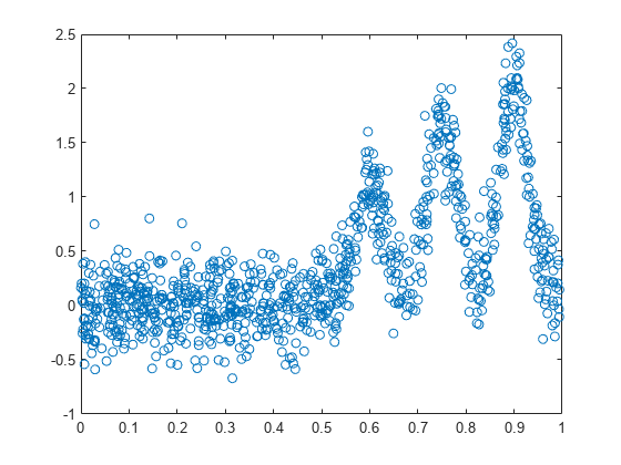
Plot $y$ versus sorted $x$ .

[x_sorted,I] = sort(x,'ascend');
plot(x_sorted,y(I),'o')

Figure contains an axes object. The axes contains a line object which displays its values using only markers.

Fit the following mixed-effects linear spline regression model

$y_{i} = β_{1} + β_{2} x_{i} + \sum_{j = 1}^{K} b_{j} {(x_{i} - k_{j})}_{+} + ϵ_{i}$

where $k_{j}$ is the $j$ th knot, and $K$ is the total number of knots. Assume that $b_{j} \sim N (0, σ_{b}^{2})$ and $ϵ \sim N (0, σ^{2})$ .

Define the knots.

k = linspace(0.05,0.95,100);

Define the design matrices.

X = [ones(1000,1),x];
Z = zeros(length(x),length(k));
for j = 1:length(k)
      Z(:,j) = max(X(:,2) - k(j),0);
end

Fit the model with an isotropic covariance structure for the random effects.

lme = fitlmematrix(X,y,Z,[],'CovariancePattern','Isotropic');

Fit a fixed-effects only model.

X = [X Z];
lme_fixed = fitlmematrix(X,y,[],[]);

Compare lme_fixed and lme via a simulated likelihood ratio test.

compare(lme,lme_fixed,'NSim',500,'CheckNesting',true)

ans = 
    SIMULATED LIKELIHOOD RATIO TEST: NSIM = 500, ALPHA = 0.05

    Model        DF     AIC       BIC       LogLik     LRStat    pValue     Lower      Upper  
    lme            4    170.62    190.25    -81.309                                           
    lme_fixed    103    113.38    618.88     46.309    255.24    0.68064    0.63784    0.72129

The $p$ -value indicates that the fixed-effects only model is not a better fit than the mixed-effects spline regression model.

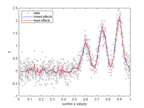
Plot the fitted values from both models on top of the original response data.

R = response(lme);
figure();
plot(x_sorted,R(I),'o', 'MarkerFaceColor',[0.8,0.8,0.8],...
    'MarkerEdgeColor',[0.8,0.8,0.8],'MarkerSize',4);
hold on
F = fitted(lme);
F_fixed = fitted(lme_fixed);
plot(x_sorted,F(I),'b');
plot(x_sorted,F_fixed(I),'r');
legend('data','mixed effects','fixed effects','Location','NorthWest')
xlabel('sorted x values');
ylabel('y');
hold off

Figure contains an axes object. The axes object with xlabel sorted x values, ylabel y contains 3 objects of type line. One or more of the lines displays its values using only markers These objects represent data, mixed effects, fixed effects.

You can also see from the figure that the mixed-effects model provides a better fit to data than the fixed-effects only model.