Implement Bayesian Binomial Regression

Open Live Script

This example fits a binomial regression model to dose-response data using Bayesian methods, including Metropolis–Hastings sampling. Also, the example shows how to set up a custom target distribution function to generate multiple independent samples (Markov chains) for a multivariate problem.

Consider the following simulated dose-response data set measuring the number of subjects experiencing at least one adverse effect within three days of receiving a dose of a drug.

Dose (log g/ml, $x_{j}$ )	Number of Subjects ( $n_{j}$ )	Number of Affected Subjects ( $y_{j}$ )
-1.4	10	1
-0.7	10	1
-0.3	10	3
0	10	8
0.4	10	9

The goal of this experiment is to estimate $p_{j}$ , the probability of someone in the population experiencing an adverse effect given dose $x_{j}$ , by fitting the logistic regression model $logit (p_{j}) = β_{0} + β_{1} x_{j}$ . Given $n_{j}$ , $p_{j}$ , and $x_{j}$ , $y_{j} | p_{j}, n_{j} \sim Binomial (n_{j}, p_{j})$ for each dose level $j$ . The problem reduces to the estimation and inferences on $β_{0}$ and $β_{1}$ .

Organize Data

Create variables for the columns of the data table.

dose = [0.25; 0.5; 0.75; 1; 1.5];
ld = log(dose);
n = 10*ones(5,1);
y = [1; 1; 3; 8; 9];

Assuming the subjects are independent of each other, one Bayesian view of this statistical problem includes the following distributions:

A noninformative joint prior distribution $π (β_{0}, β_{1}) \propto 1$ .
The likelihood function $P (y_{j} | n_{j}, β_{0}, β_{1}, x_{j}) \propto {[{logit}^{- 1} (β_{0} + β_{1} x_{j})]}^{y_{j}} {[{1 - logit}^{- 1} (β_{0} + β_{1} x_{j})]}^{n_{j} - y_{j}}$ .
The posterior distribution $π_{j} (β_{0}, β_{1} | y_{j}) \propto π (β_{0,} β_{1}) \prod_{j} P (y_{j} | n_{j}, β_{0}, β_{1}, x_{j})$ .

Assign Posterior as Target PDF

Create a function that computes the log of an expression that is proportional to the posterior. Write the function so that it accepts a matrix of starting values for $β = {[\begin{array}{c} β_{0} & β_{1} \end{array}]}^{'}$ , and each starting value initializes a separate, independently generated Markov chain. Each column represents a coefficient, and each row is a separate set of starting values for the coefficients. The function returns a numeric column vector of pdf evaluations for each independently generated Markov chain.

priorBeta = 1;                                  % Prior distribution
p = @(beta,x)(([ones(height(x),1) x]*beta'))';  % Linear combination of coefficients and predictor
invlogit = @(t)exp(t)./(1+exp(t));              % Inverse logit function
logLH = @(beta,x,y,n)(y'.*log(invlogit(p(beta,x))) + (n-y)'.*log(1-invlogit(p(beta,x)))); % Dose-wise loglikelihood
targetLogPDF = @(beta)log(priorBeta) + sum(logLH(beta,ld,y,n),2);

This example generates 25 independent Markov chains. Verify that the target log pdf returns the correct evaluations in the correct form.

numbeta = 2;
numchains = 25;
rng(1,"twister")
testbeta = randn(numchains,numbeta);
testpdf1 = targetLogPDF(testbeta);
testpdf2 = nan(numchains,1);
for j = 1:numchains
    testpdf2(j) = targetLogPDF(testbeta(j,:));
end
size(testpdf1) == [numchains 1]

ans = 1×2 logical array

   1   1

(testpdf1 - testpdf2)'*(testpdf1 - testpdf2) <= eps

ans = logical
   1

targetLogPDF returns the correct log pdf values in the correct form.

Generate Markov Chains Using Metropolis–Hastings Sampler

Generate 25 independent samples (Markov chains) from the posterior distribution using the Random-Walk Metropolis–Hastings sampler with the following settings:

Specify length 1000 Markov chains (per-chain sample size).
Specify the Student's $t$ proposal with a scale matrix, a two-dimensional identity matrix, and 5 degrees of freedom.
Initialize each chain using two randomly drawn values from a standard Gaussian distribution.
Specify a burn-in period of 500.
Specify a thinning factor of 10.

Return the acceptance rate of each generated Markov chain.

numsamples = 1000;
scale = eye(numbeta);
dof = 5;
start = randn(numchains,numbeta);
burnin = 500;
thin = 10;

[sample,acceptance] = mhsample(start,numsamples,LogPDF=targetLogPDF,NumChains=numchains, ...
    Proposal="t",Scale=scale,DegreesOfFreedom=dof,Thin=thin,BurnIn=burnin);

sample is a 1000-by-2-by-25 array of generated samples. Each page is an independently generated, length 1000 posterior sample from the joint distribution of $β$ . acceptance is a 25-by-1 vector of proposal acceptance rates corresponding to the Markov chains.

Diagnose Samples

Determine how sensitive the sampler is to the initial values by, computing and plotting the average and standard deviation for each chain.

ave = squeeze(mean(sample,1));
sd = squeeze(std(sample,0,1));

figure
tiledlayout(2,1)
nexttile;
yyaxis left
plot(ave(1,:))
yyaxis right
plot(sd(1,:))
legend("Mean","Standard deviation")
title("Estimated Posterior Moments: \beta_0")
nexttile;
yyaxis left
plot(ave(2,:))
yyaxis right
plot(sd(2,:))
legend("Mean","Standard deviation")
title("Estimated Posterior Moments: \beta_1")

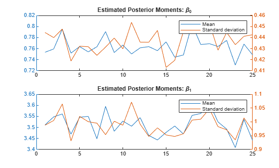
Figure contains 2 axes objects. Axes object 1 with title Estimated Posterior Moments: beta indexOf 0 baseline contains an object of type line. These objects represent Mean, Standard deviation. Axes object 2 with title Estimated Posterior Moments: beta indexOf 1 baseline contains an object of type line. These objects represent Mean, Standard deviation.

The estimated posterior moments appear stable.

Plot the acceptance rates of the chains.

figure
plot(acceptance)
title("Acceptance Rates")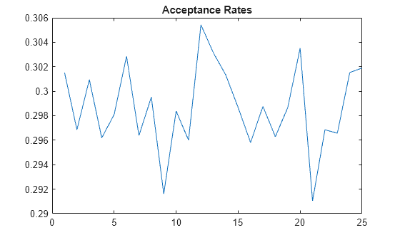

Figure contains an axes object. The axes object with title Acceptance Rates contains an object of type line.

The acceptance rate series is stable, fluctuating around 0.3, which is an acceptable rate.

Create a time series plot of the first posterior sample.

figure
tiledlayout(2,1)
nexttile;
plot(sample(:,1,1))
title("First Posterior Sample: \beta_0")
nexttile;
plot(sample(:,2,1))
title("First Posterior Sample: \beta_1")

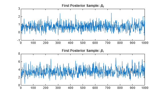
Figure contains 2 axes objects. Axes object 1 with title First Posterior Sample: beta indexOf 0 baseline contains an object of type line. Axes object 2 with title First Posterior Sample: beta indexOf 1 baseline contains an object of type line.

The sample appears to mix adequately, with small serial correlation and little transient behavior.

Estimate Posterior Probabilities of Adverse Events

For each dose level, obtain a posterior sample of the probability of an adverse effect by applying the inverse logit function to the linear combination of each sampled set of coefficients and log dose.

MC1 = sample(:,:,1);
postprob = invlogit(p(MC1,ld));

postprob is a 1000-by-5 matrix of samples from the joint distribution of the probabilities of adverse effects among the dose levels.

Compute the mean of each posterior sample, which is the expected probability of an adverse effect.

meanpost = mean(postprob);
table(dose,meanpost',VariableName=["Dose" "Prob. Adverse Effect"])

ans=5×2 table
    Dose    Prob. Adverse Effect
    ____    ____________________

    0.25          0.027698      
     0.5            0.1717      
    0.75           0.43846      
       1            0.6726      
     1.5            0.8795

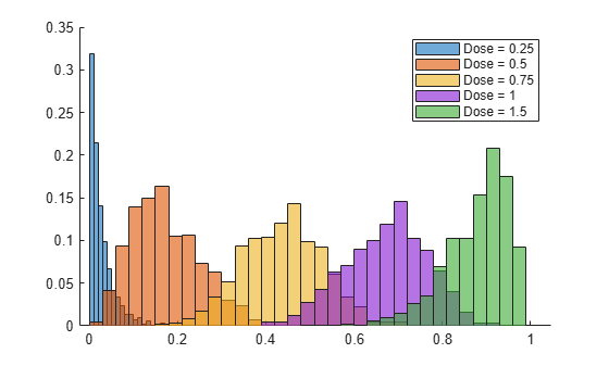
Plot a histogram showing the posterior distribution of the probability of an adverse effect for each dose level.

figure
hold on
for j = 1:width(postprob)
    histogram(postprob(:,j),Normalization="probability")
end
hold off
legend("Dose = " + string(dose))

Figure contains an axes object. The axes object contains 5 objects of type histogram. These objects represent Dose = 0.25, Dose = 0.5, Dose = 0.75, Dose = 1, Dose = 1.5.

Compare Coefficient Estimates with Using Classic Approach

The classic approach to this type of problem is to fit a generalized linear model with a logit link to the data.

Estimate the coefficients by using fitglm.

resp = [y n];
mdl = fitglm(ld,resp,"linear",Distribution="binomial")

mdl = 
Generalized linear regression model:
    logit(y) ~ 1 + x1
    Distribution = Binomial

Estimated Coefficients:
                   Estimate      SE       tStat       pValue  
                   ________    _______    ______    __________

    (Intercept)    0.70286     0.41835    1.6801      0.092942
    x1              3.1936     0.92275     3.461    0.00053814


5 observations, 3 error degrees of freedom
Dispersion: 1
Chi^2-statistic vs. constant model: 23.1, p-value = 1.5e-06

The classic estimates are close to the Bayesian estimates.