Linear Mixed-Effects Model Workflow
This example shows how to fit and analyze a linear mixed-effects model (LME).
Load the sample data.
load flu
The flu dataset array has a Date variable, and 10 variables containing estimated influenza rates (in 9 different regions, estimated from Google® searches, plus a nationwide estimate from the CDC).
Reorganize and plot the data.
To fit a linear-mixed effects model, your data must be in a properly formatted table. To fit a linear mixed-effects model with the influenza rates as the responses, combine the nine columns corresponding to the regions into an array. The new dataset array, flu2, must have the response variable FluRate, the nominal variable Region that shows which region each estimate is from, the nationwide estimate WtdILI, and the grouping variable Date.
flu2 = stack(flu,2:10,'NewDataVarName','FluRate',...
    'IndVarName','Region');
flu2.Date = nominal(flu2.Date);
Define flu2 as a table.
flu2 = dataset2table(flu2);
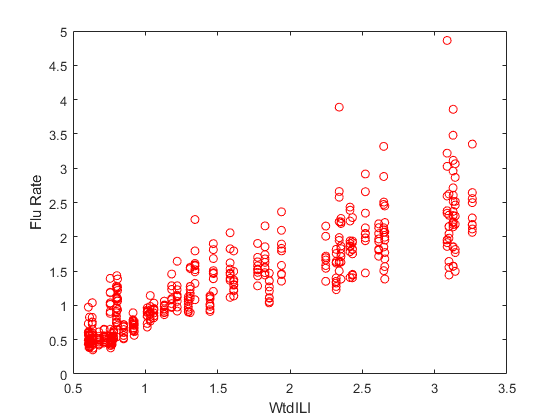
Plot flu rates versus the nationwide estimate.
plot(flu2.WtdILI,flu2.FluRate,'ro')
xlabel('WtdILI')
ylabel('Flu Rate')

You can see that the flu rates in regions have a direct relationship with the nationwide estimate.
Fit an LME model and interpret the results.
Fit a linear mixed-effects model with the nationwide estimate as the predictor variable and a random intercept that varies by Date.
lme = fitlme(flu2,'FluRate ~ 1 + WtdILI + (1|Date)')
lme =


Linear mixed-effects model fit by ML

Model information:
    Number of observations             468
    Fixed effects coefficients           2
    Random effects coefficients         52
    Covariance parameters                2

Formula:
    FluRate ~ 1 + WtdILI + (1 | Date)

Model fit statistics:
    AIC       BIC       LogLikelihood    Deviance
    286.24    302.83    -139.12          278.24

Fixed effects coefficients (95% CIs):
    Name                   Estimate    SE          tStat     DF     pValue
    {'(Intercept)'}        0.16385     0.057525    2.8484    466     0.0045885
    {'WtdILI'     }         0.7236     0.032219    22.459    466    3.0502e-76


    Lower       Upper
    0.050813    0.27689
     0.66028    0.78691

Random effects covariance parameters (95% CIs):
Group: Date (52 Levels)
    Name1                  Name2                  Type           Estimate
    {'(Intercept)'}        {'(Intercept)'}        {'std'}        0.17146


    Lower      Upper
    0.13227    0.22226

Group: Error
    Name               Estimate    Lower      Upper
    {'Res Std'}        0.30201     0.28217    0.32324
The small  -values of 0.0045885 and 3.0502e-76 indicate that both the intercept and nationwide estimate are significant. Also, the confidence limits for the standard deviation of the random-effects term,
  , do not include 0 (0.13227, 0.22226), which indicates that the random-effects term is significant.
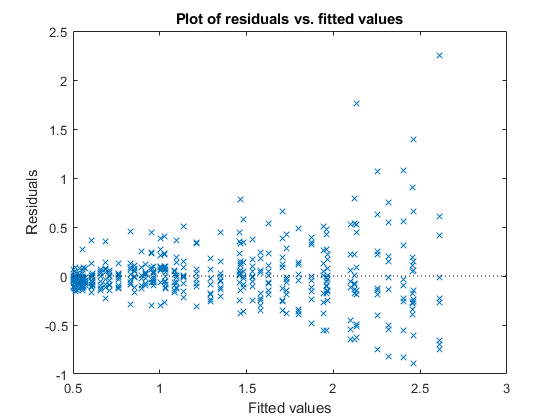
Plot the raw residuals versus the fitted values.
figure();
plotResiduals(lme,'fitted')

The variance of residuals increases with increasing fitted response values, which is known as heteroscedasticity.
Find the two observations on the top right that appear like outliers.
find(residuals(lme) > 1.5)
ans =

    98
   107
Refit the model by removing these observations.
lme = fitlme(flu2,'FluRate ~ 1 + WtdILI + (1|Date)','Exclude',[98,107]);
Improve the model.
Determine if including an independent random term for the nationwide estimate grouped by Date improves the model.
altlme = fitlme(flu2,'FluRate ~ 1 + WtdILI + (1|Date) + (WtdILI-1|Date)',...
'Exclude',[98,107])
altlme =


Linear mixed-effects model fit by ML

Model information:
    Number of observations             466
    Fixed effects coefficients           2
    Random effects coefficients        104
    Covariance parameters                3

Formula:
    FluRate ~ 1 + WtdILI + (1 | Date) + (WtdILI | Date)

Model fit statistics:
    AIC       BIC       LogLikelihood    Deviance
    179.39    200.11    -84.694          169.39

Fixed effects coefficients (95% CIs):
    Name                   Estimate    SE          tStat     DF     pValue
    {'(Intercept)'}        0.17837     0.054585    3.2676    464     0.001165
    {'WtdILI'     }        0.70836     0.030594    23.153    464    2.123e-79


    Lower      Upper
     0.0711    0.28563
    0.64824    0.76849

Random effects covariance parameters (95% CIs):
Group: Date (52 Levels)
    Name1                  Name2                  Type           Estimate
    {'(Intercept)'}        {'(Intercept)'}        {'std'}        0.16631


    Lower      Upper
    0.12977    0.21313

Group: Date (52 Levels)
    Name1             Name2             Type           Estimate      Lower
    {'WtdILI'}        {'WtdILI'}        {'std'}        4.6899e-08    NaN


    Upper
    NaN

Group: Error
    Name               Estimate    Lower      Upper
    {'Res Std'}        0.26691     0.24934    0.28572
The estimated standard deviation of WtdILI term is nearly 0 and its confidence interval cannot be computed. This is an indication that the model is overparameterized and the (WtdILI-1|Date) term is not significant. You can formally test this using the compare method as follows: compare(lme,altlme,'CheckNesting',true).
Add a random effects-term for intercept grouped by Region to the initial model lme.
lme2 = fitlme(flu2,'FluRate ~ 1 + WtdILI + (1|Date) + (1|Region)',...
'Exclude',[98,107]);
Compare the models lme and lme2.
compare(lme,lme2,'CheckNesting',true)
ans =


    THEORETICAL LIKELIHOOD RATIO TEST

    Model    DF    AIC       BIC       LogLik     LRStat    deltaDF    pValue
    lme      4     177.39    193.97    -84.694
    lme2     5     62.265    82.986    -26.133    117.12    1          0
The  -value of 0 indicates that
 lme2 is a better fit than lme.
Now, check if adding a potentially correlated random-effects term for the intercept and national average improves the model lme2.
lme3 = fitlme(flu2,'FluRate ~ 1 + WtdILI + (1|Date) + (1 + WtdILI|Region)',...
'Exclude',[98,107])
lme3 =


Linear mixed-effects model fit by ML

Model information:
    Number of observations             466
    Fixed effects coefficients           2
    Random effects coefficients         70
    Covariance parameters                5

Formula:
    FluRate ~ 1 + WtdILI + (1 | Date) + (1 + WtdILI | Region)

Model fit statistics:
    AIC       BIC       LogLikelihood    Deviance
    13.338    42.348    0.33076          -0.66153

Fixed effects coefficients (95% CIs):
    Name                   Estimate    SE          tStat     DF     pValue
    {'(Intercept)'}         0.1795     0.054953    3.2665    464     0.0011697
    {'WtdILI'     }        0.70719      0.04252    16.632    464    4.6451e-49


    Lower       Upper
    0.071514    0.28749
     0.62363    0.79074

Random effects covariance parameters (95% CIs):
Group: Date (52 Levels)
    Name1                  Name2                  Type           Estimate
    {'(Intercept)'}        {'(Intercept)'}        {'std'}        0.17634


    Lower      Upper
    0.14093    0.22064

Group: Region (9 Levels)
    Name1                  Name2                  Type            Estimate
    {'(Intercept)'}        {'(Intercept)'}        {'std' }        0.0077038
    {'WtdILI'     }        {'(Intercept)'}        {'corr'}        -0.059604
    {'WtdILI'     }        {'WtdILI'     }        {'std' }         0.088069


    Lower         Upper
    3.2005e-16    1.8543e+11
      -0.99996       0.99995
      0.051693       0.15004

Group: Error
    Name               Estimate    Lower      Upper
    {'Res Std'}        0.20976     0.19568    0.22486
The estimate for the standard deviation of the random-effects term for intercept grouped by Region is 0.0077037, its confidence interval is very large and includes zero. This indicates that the random-effects for intercept grouped by Region is insignificant. The correlation between the random-effects for intercept and WtdILI is -0.059604. Its confidence interval is also very large and includes zero. This is an indication that the correlation is not significant.
Refit the model by eliminating the intercept from the (1 + WtdILI | Region) random-effects term.
lme3 = fitlme(flu2,'FluRate ~ 1 + WtdILI + (1|Date) + (WtdILI - 1|Region)',...
'Exclude',[98,107])
lme3 =


Linear mixed-effects model fit by ML

Model information:
    Number of observations             466
    Fixed effects coefficients           2
    Random effects coefficients         61
    Covariance parameters                3

Formula:
    FluRate ~ 1 + WtdILI + (1 | Date) + (WtdILI | Region)

Model fit statistics:
    AIC       BIC      LogLikelihood    Deviance
    9.3395    30.06    0.33023          -0.66046

Fixed effects coefficients (95% CIs):
    Name                   Estimate    SE          tStat     DF     pValue
    {'(Intercept)'}         0.1795     0.054892    3.2702    464     0.0011549
    {'WtdILI'     }        0.70718     0.042486    16.645    464    4.0496e-49


    Lower       Upper
    0.071637    0.28737
     0.62369    0.79067

Random effects covariance parameters (95% CIs):
Group: Date (52 Levels)
    Name1                  Name2                  Type           Estimate
    {'(Intercept)'}        {'(Intercept)'}        {'std'}        0.17633


    Lower      Upper
    0.14092    0.22062

Group: Region (9 Levels)
    Name1             Name2             Type           Estimate    Lower
    {'WtdILI'}        {'WtdILI'}        {'std'}        0.087925    0.054474


    Upper
    0.14192

Group: Error
    Name               Estimate    Lower      Upper
    {'Res Std'}        0.20979     0.19585    0.22473
All terms in the new model lme3 are significant.
Compare lme2 and lme3.
compare(lme2,lme3,'CheckNesting',true,'NSim',100)
ans =


    SIMULATED LIKELIHOOD RATIO TEST: NSIM = 100, ALPHA = 0.05

    Model    DF    AIC       BIC       LogLik     LRStat    pValue
    lme2     5     62.265    82.986    -26.133
    lme3     5     9.3395     30.06    0.33023    52.926    0.009901


    Lower         Upper

    0.00025064    0.053932
The  -value of 0.009901 indicates that
 lme3 is a better fit than lme2.
Add a quadratic fixed-effects term to the model lme3.
lme4 = fitlme(flu2,'FluRate ~ 1 + WtdILI^2 + (1|Date) + (WtdILI - 1|Region)',...
'Exclude',[98,107])
lme4 =


Linear mixed-effects model fit by ML

Model information:
    Number of observations             466
    Fixed effects coefficients           3
    Random effects coefficients         61
    Covariance parameters                3

Formula:
    FluRate ~ 1 + WtdILI + WtdILI^2 + (1 | Date) + (WtdILI | Region)

Model fit statistics:
    AIC       BIC       LogLikelihood    Deviance
    6.7234    31.588    2.6383           -5.2766

Fixed effects coefficients (95% CIs):
    Name                   Estimate     SE         tStat       DF     pValue
    {'(Intercept)'}        -0.063406    0.12236    -0.51821    463       0.60456
    {'WtdILI'     }           1.0594    0.16554      6.3996    463    3.8232e-10
    {'WtdILI^2'   }        -0.096919     0.0441     -2.1977    463      0.028463


    Lower       Upper
    -0.30385      0.17704
     0.73406       1.3847
    -0.18358    -0.010259

Random effects covariance parameters (95% CIs):
Group: Date (52 Levels)
    Name1                  Name2                  Type           Estimate
    {'(Intercept)'}        {'(Intercept)'}        {'std'}        0.16732


    Lower      Upper
    0.13326    0.21009

Group: Region (9 Levels)
    Name1             Name2             Type           Estimate    Lower
    {'WtdILI'}        {'WtdILI'}        {'std'}        0.087865    0.054443


    Upper
    0.1418

Group: Error
    Name               Estimate    Lower      Upper
    {'Res Std'}        0.20979     0.19585    0.22473
The  -value of 0.028463 indicates that the coefficient of the quadratic term
 WtdILI^2 is significant.
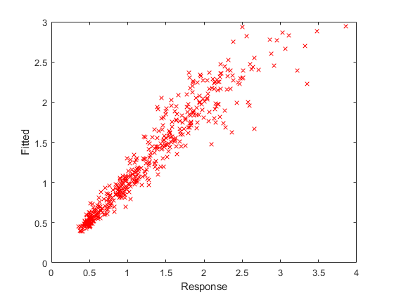
Plot the fitted response versus the observed response and residuals.
F = fitted(lme4);
R = response(lme4);
figure();
plot(R,F,'rx')
xlabel('Response')
ylabel('Fitted')

The fitted versus observed response values form almost 45-degree angle indicating a good fit.
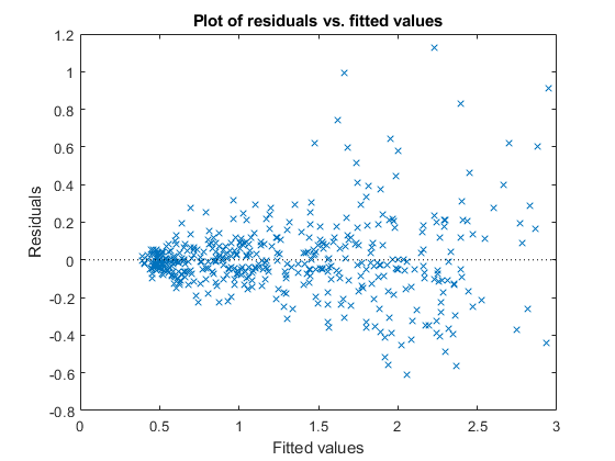
Plot the residuals versus the fitted values.
figure();
plotResiduals(lme4,'fitted')

Although it has improved, you can still see some heteroscedasticity in the model. This might be due to another predictor that does not exist in the data set, hence not in the model.
Find the fitted flu rate value for region ENCentral, date 11/6/2005.
F(flu2.Region == 'ENCentral' & flu2.Date == '11/6/2005')
ans =

    1.4860
Randomly generate response values.
Randomly generate response values for a national estimate of 1.625, region MidAtl, and date 4/23/2006. First, define the new table. Because Date and Region are nominal in the original table, you must define them similarly in the new table.
tblnew.Date = nominal('4/23/2006');
tblnew.WtdILI = 1.625;
tblnew.Region = nominal('MidAtl');
tblnew = struct2table(tblnew);
Now, generate the response value.
random(lme4,tblnew)
ans =

    1.2679