Perform Accelerated Life Model Analysis

Load and Visualize Data

Load the machineFailure data set, which contains 100 simulated failure time measurements of the machine part at five evenly spaced temperatures (T) between 300 K and 400 K. Approximately 5% of the failure time measurements are right-censored. These measurements are indicated in the censored variable of the table.

load machineFailure

Create a histogram of the failure times at the lowest stressor level in the data set (T = 300).

histogram(failureTable.failureTime(failureTable.T==300),BinWidth=2)
xlabel("Failure Time");
title("Failure Times at T = 300 K")

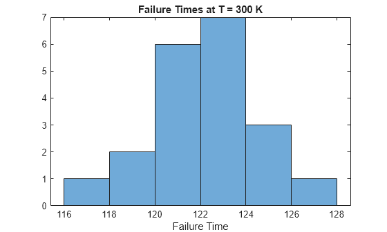
The histogram shows that the failure times at the first stressor level are approximately normally distributed.

Create a plot of mean failure time versus stressor level.

s = groupsummary(failureTable,"T","mean","failureTime");
plot(s.T,s.mean_failureTime,"-o")
xlabel("T")
ylabel("Failure Time");

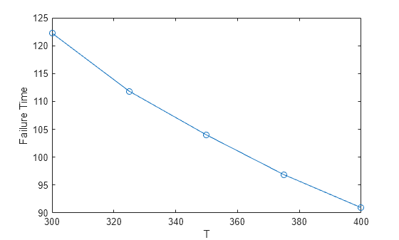
The plot indicates that the mean failure time has a nonlinear dependence on temperature. The failure times in this data set follow an Eyring relationship, which has the functional form f(T) = 1/T*exp(–(b0–b1/T)), where b0 and b1 are model coefficients.

Fit Accelerated Life Model

Fit an accelerated life model to the data using the fitacclife function. Specify a normal life distribution and an Eyring life stress model. Use 230 K as the baseline stressor level.

mdl = fitacclife(failureTable,"failureTime", ...
    Censoring=failureTable.censored,Distribution="normal", ...
    StressModel="eyring",StressorName="T",BaselineStressorLevel=230)

mdl = 
AcceleratedLifeModel

Life distribution: normal
Stress model: eyring
Baseline stressor level: 230

     T     NormalMu    MeanFailureTime    AccelerationFactor
    ___    ________    _______________    __________________

    400     90.742         90.742               1.7712      
    375     96.951         96.951               1.6577      
    350     104.07         104.07               1.5443      
    325     112.32         112.32               1.4309      
    300     121.99         121.99               1.3175      
    230     160.72         160.72                    1      


Log-likelihood: -195.5267

mdl is an AcceleratedLifeModel object, which you can use to compute mean failure times, calculate failure probabilities at specific stressor levels, and create plots. The first column of the output contains the unique stressor levels in the data and the baseline stressor level. The second and third columns list the fitted life distribution parameter values and mean failure times, respectively. The fourth column lists the acceleration factor, which is the ratio of the mean failure time at the stressor level to the mean failure time at the baseline stressor level.

Display information about the fitted model coefficients.

mdl.Coefficients

ans=3×3 table
                       Source        Estimate       SE   
                   ______________    ________    ________

    b0             "StressModel"     -10.475     0.016919
    b1             "StressModel"      9.8762        5.709
    NormalSigma    "Distribution"     1.7779      0.13054

The table lists the estimated value and the standard error of each coefficient in the life stress model, and the estimated value and the standard error of the life distribution parameter. The life distribution parameter (NormalSigma) and the first coefficient (b0) of the life stress model are well constrained. The second coefficient of the life stress model (b1) is not well constrained.

List the 95% confidence intervals for each fitted model coefficient and parameter.

coefci(mdl)

ans = 3×2

  -10.5084  -10.4412
   -1.4545   21.2070
    1.5188    2.0370

Display the mean failure times according to the model.

meanfailtime(mdl)

ans=6×2 table
     T     MeanFailureTime
    ___    _______________

    400        90.742     
    375        96.951     
    350        104.07     
    325        112.32     
    300        121.99     
    230        160.72     

The last row in the table indicates that the mean failure time at the baseline stressor level (T = 230) is 160.7.

Create a plot of the mean failure times.

meanfailplot(mdl)

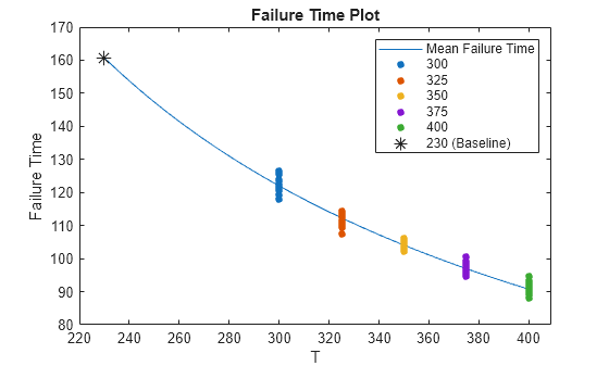
The plot indicates that the Eyring model provides a good fit to the mean failure times at different stressor levels. The mean predicted failure time at the baseline stressor level is indicated on the plot with an asterisk marker.

Create a probability plot of the model and the data.

probplot(mdl)

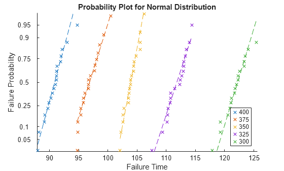
The log-linear plot shows each observation in the data, grouped by stressor level. Each dashed reference line connects the first and third quartiles of the failure time data for that stressor level and extends to the ends of the data. The failure times are shorter at higher temperatures. Also, at a fixed stressor level, the failure probability increases nonlinearly with time.