Perform Text Classification Incrementally
This example shows how to incrementally train a model to classify documents based on word frequencies in the documents; a bag-of-words model.
Load the NLP data set, which contains a sparse matrix of word frequencies X computed from MathWorks® documentation. Labels Y are the toolbox documentation to which the page belongs.
load nlpdataFor more details on the data set, such as the dictionary and corpus, enter Description.
The observations are arranged by label. Because the incremental learning software does not start computing performance metrics until it processes all labels at least once, shuffle the data set.
[n,p] = size(X)
n = 31572
p = 34023
rng(1);
shflidx = randperm(n);
X = X(shflidx,:);
Y = Y(shflidx);
Determine the number of classes in the data.
cats = categories(Y);
maxNumClasses = numel(cats);
Create a naive Bayes incremental learner. Specify the number of classes, a metrics warmup period of 0, and a metrics window size of 1000. Because predictor is the word frequency of word in the dictionary, specify that the predictors are conditionally, jointly multinomial, given the class.
Mdl = incrementalClassificationNaiveBayes(MaxNumClasses=maxNumClasses,...
    MetricsWarmupPeriod=0,MetricsWindowSize=1000,DistributionNames='mn');
Mdl is an incrementalClassificationNaiveBayes object. Mdl is a cold model because it has not processed observation; it represents a template for training.
Measure the model performance and fit the incremental model to the training data by using the updateMetricsAndFit function. Simulate a data stream by processing chunks of 1000 observations at a time. At each iteration:
Process 1000 observations.
Overwrite the previous incremental model with a new one fitted to the incoming observations.
Store the current minimal cost.
This stage can take several minutes to run.
numObsPerChunk = 1000;
nchunks = floor(n/numObsPerChunk);
mc = array2table(zeros(nchunks,2),'VariableNames',["Cumulative" "Window"]);

for j = 1:nchunks
    ibegin = min(n,numObsPerChunk*(j-1) + 1);
    iend   = min(n,numObsPerChunk*j);
    idx = ibegin:iend;
    XChunk = full(X(idx,:));
    Mdl = updateMetricsAndFit(Mdl,XChunk,Y(idx));
    mc{j,:} = Mdl.Metrics{"MinimalCost",:};
end
Mdl is an incrementalClassificationNaiveBayes model object trained on all the data in the stream. During incremental learning and after the model is warmed up, updateMetricsAndFit checks the performance of the model on the incoming chunk of observations, and then fits the model to those observations.
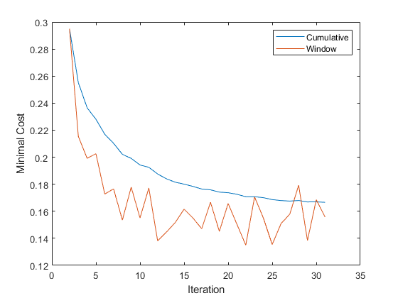
Plot the minimal cost to see how it evolved during training.
figure
plot(mc.Variables)
ylabel('Minimal Cost')
legend(mc.Properties.VariableNames)
xlabel('Iteration')

The cumulative minimal cost smoothly decreases and settles near 0.16, while the minimal cost computed for the chunk jumps between 0.14 and 0.18.
See Also
Objects
Functions
predict|fit|updateMetrics