Pitfalls in Fitting Nonlinear Models by Transforming to Linearity

This example shows pitfalls that can occur when fitting a nonlinear model by transforming to linearity. Imagine that we have collected measurements on two variables, x and y, and we want to model y as a function of x. Assume that x is measured exactly, while measurements of y are affected by additive, symmetric, zero-mean errors.

x = [5.72 4.22 5.72 3.59 5.04 2.66 5.02 3.11 0.13 2.26 ...
     5.39 2.57 1.20 1.82 3.23 5.46 3.15 1.84 0.21 4.29 ...
     4.61 0.36 3.76 1.59 1.87 3.14 2.45 5.36 3.44 3.41]';
y = [2.66 2.91 0.94 4.28 1.76 4.08 1.11 4.33 8.94 5.25 ...
     0.02 3.88 6.43 4.08 4.90 1.33 3.63 5.49 7.23 0.88 ...
     3.08 8.12 1.22 4.24 6.21 5.48 4.89 2.30 4.13 2.17]';

Let's also assume that theory tells us that these data should follow a model of exponential decay, y = p1*exp(p2*x), where p1 is positive and p2 is negative. To fit this model, we could use nonlinear least squares.

modelFun = @(p,x) p(1)*exp(p(2)*x);

But the nonlinear model can also be transformed to a linear one by taking the log on both sides, to get log(y) = log(p1) + p2*x. That's tempting, because we can fit that linear model by ordinary linear least squares. The coefficients we'd get from a linear least squares would be log(p1) and p2.

paramEstsLin = [ones(size(x)), x] \ log(y);
paramEstsLin(1) = exp(paramEstsLin(1))

paramEstsLin =

   11.9312
   -0.4462

How did we do? We can superimpose the fit on the data to find out.

xx = linspace(min(x), max(x));
yyLin = modelFun(paramEstsLin, xx);
plot(x,y,'o', xx,yyLin,'-');
xlabel('x'); ylabel('y');
legend({'Raw data','Linear fit on the log scale'},'location','NE');

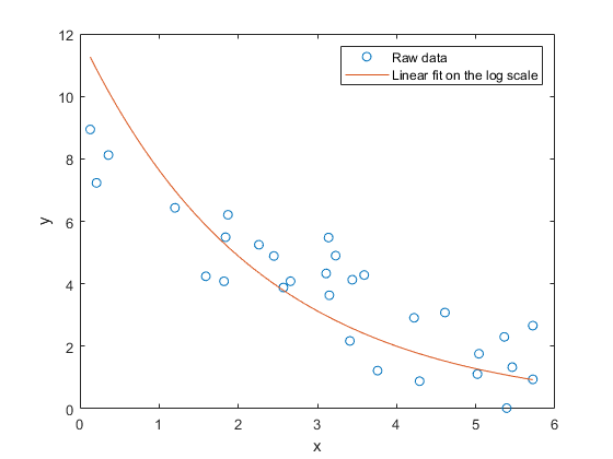
Something seems to have gone wrong, because the fit doesn't really follow the trend that we can see in the raw data. What kind of fit would we get if we used nlinfit to do nonlinear least squares instead? We'll use the previous fit as a rough starting point, even though it's not a great fit.

paramEsts = nlinfit(x, y, modelFun, paramEstsLin)

paramEsts =

    8.8145
   -0.2885

yy = modelFun(paramEsts,xx);
plot(x,y,'o', xx,yyLin,'-', xx,yy,'-');
xlabel('x'); ylabel('y');
legend({'Raw data','Linear fit on the log scale',  ...
	'Nonlinear fit on the original scale'},'location','NE');

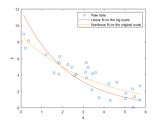
The fit using nlinfit more or less passes through the center of the data point scatter. A residual plot shows something approximately like an even scatter about zero.

r = y-modelFun(paramEsts,x);
plot(x,r,'+', [min(x) max(x)],[0 0],'k:');
xlabel('x'); ylabel('residuals');

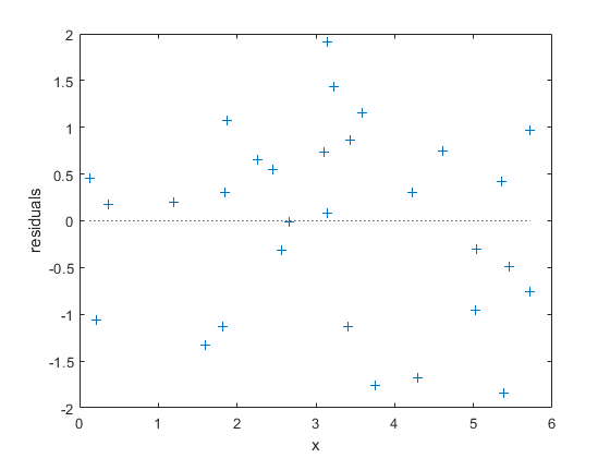
So what went wrong with the linear fit? The problem is in log transform. If we plot the data and the two fits on the log scale, we can see that there's an extreme outlier.

plot(x,log(y),'o', xx,log(yyLin),'-', xx,log(yy),'-');
xlabel('x'); ylabel('log(y)');
ylim([-5,3]);
legend({'Raw data', 'Linear fit on the log scale',  ...
	'Nonlinear fit on the original scale'},'location','SW');

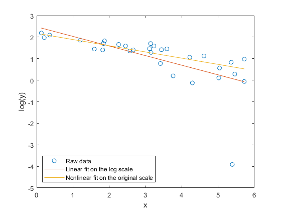
That observation is not an outlier in the original data, so what happened to make it one on the log scale? The log transform is exactly the right thing to straighten out the trend line. But the log is a very nonlinear transform, and so symmetric measurement errors on the original scale have become asymmetric on the log scale. Notice that the outlier had the smallest y value on the original scale -- close to zero. The log transform has "stretched out" that smallest y value more than its neighbors. We made the linear fit on the log scale, and so it is very much affected by that outlier.

Had the measurement at that one point been slightly different, the two fits might have been much more similar. For example,

y(11) = 1;
paramEsts = nlinfit(x, y, modelFun, [10;-.3])

paramEsts =

    8.7618
   -0.2833

paramEstsLin = [ones(size(x)), x] \ log(y);
paramEstsLin(1) = exp(paramEstsLin(1))

paramEstsLin =

    9.6357
   -0.3394

yy = modelFun(paramEsts,xx);
yyLin = modelFun(paramEstsLin, xx);
plot(x,y,'o', xx,yyLin,'-', xx,yy,'-');
xlabel('x'); ylabel('y');
legend({'Raw data', 'Linear fit on the log scale',  ...
	'Nonlinear fit on the original scale'},'location','NE');

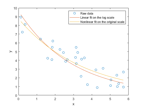
Still, the two fits are different. Which one is "right"? To answer that, suppose that instead of additive measurement errors, measurements of y were affected by multiplicative errors. These errors would not be symmetric, and least squares on the original scale would not be appropriate. On the other hand, the log transform would make the errors symmetric on the log scale, and the linear least squares fit on that scale is appropriate.

So, which method is "right" depends on what assumptions you are willing to make about your data. In practice, when the noise term is small relative to the trend, the log transform is "locally linear" in the sense that y values near the same x value will not be stretched out too asymmetrically. In that case, the two methods lead to essentially the same fit. But when the noise term is not small, you should consider what assumptions are realistic, and choose an appropriate fitting method.