Predict Responses Using RegressionEnsemble Predict Block

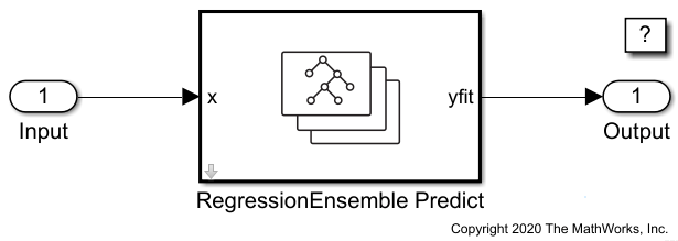
This example uses:

This example shows how to train an ensemble model with optimal hyperparameters, and then use the RegressionEnsemble Predict block for response prediction in Simulink®. The block accepts an observation (predictor data) and returns the predicted response for the observation using the trained regression ensemble model.

Train Regression Model with Optimal Hyperparameters

Load the carbig data set, which contains measurements of cars made in the 1970s and early 1980s.

load carbig
whos

  Name                Size            Bytes  Class     Attributes

  Acceleration      406x1              3248  double              
  Cylinders         406x1              3248  double              
  Displacement      406x1              3248  double              
  Horsepower        406x1              3248  double              
  MPG               406x1              3248  double              
  Mfg               406x13            10556  char                
  Model             406x36            29232  char                
  Model_Year        406x1              3248  double              
  Origin            406x7              5684  char                
  Weight            406x1              3248  double              
  cyl4              406x5              4060  char                
  org               406x7              5684  char                
  when              406x5              4060  char

Origin is a categorical variable. When you train a model for the RegressionEnsemble Predict block, you must preprocess categorical predictors by using the dummyvar function to include the categorical predictors in the model. You cannot use the 'CategoricalPredictors' name-value argument. Create dummy variables for Origin.

c_Origin = categorical(cellstr(Origin));
d_Origin = dummyvar(c_Origin);

dummyvar creates dummy variables for each category of c_Origin. Determine the number of categories in c_Origin and the number of dummy variables in d_Origin.

unique(cellstr(Origin))

ans = 7x1 cell
    {'England'}
    {'France' }
    {'Germany'}
    {'Italy'  }
    {'Japan'  }
    {'Sweden' }
    {'USA'    }

size(d_Origin)

ans = 1×2

   406     7

dummyvar creates dummy variables for each category of Origin.

Create a matrix containing six numeric predictor variables and the seven dummy variables for Origin. Also, create a vector of the response variable.

X = [Acceleration,Cylinders,Displacement,Horsepower,Model_Year,Weight,d_Origin];
Y = MPG;

Train an ensemble using X and Y with these options:

Specify 'OptimizeHyperparameters' as 'auto' to train an ensemble with optimal hyperparameters. The 'auto' option finds optimal values for 'Method','NumLearningCycles', and 'LearnRate' (for applicable methods) of fitrensemble and 'MinLeafSize' of tree learners.
For reproducibility, set the random seed and use the 'expected-improvement-plus' acquisition function. Also, for reproducibility of the random forest algorithm, specify 'Reproducible' as true for tree learners.

rng('default')
t = templateTree('Reproducible',true);
ensMdl = fitrensemble(X,Y,'Learners',t, ...
    'OptimizeHyperparameters','auto', ...
    'HyperparameterOptimizationOptions', ...
    struct('AcquisitionFunctionName','expected-improvement-plus'))

|===================================================================================================================================|
| Iter | Eval   | Objective:  | Objective   | BestSoFar   | BestSoFar   |       Method | NumLearningC-|    LearnRate |  MinLeafSize |
|      | result | log(1+loss) | runtime     | (observed)  | (estim.)    |              | ycles        |              |              |
|===================================================================================================================================|
|    1 | Best   |      2.7403 |      4.4859 |      2.7403 |      2.7403 |          Bag |          184 |            - |           69 |
|    2 | Accept |      4.1317 |     0.55941 |      2.7403 |      2.8143 |          Bag |           10 |            - |          176 |
|    3 | Best   |      2.1687 |      8.7976 |      2.1687 |      2.1689 |          Bag |          118 |            - |            2 |
|    4 | Accept |      2.2747 |      1.6637 |      2.1687 |      2.1688 |      LSBoost |           24 |      0.37779 |            7 |
|    5 | Best   |      2.1421 |      2.5588 |      2.1421 |      2.1422 |          Bag |           75 |            - |            1 |
|    6 | Best   |      2.1365 |      11.536 |      2.1365 |      2.1365 |          Bag |          500 |            - |            1 |
|    7 | Accept |      2.4302 |     0.79434 |      2.1365 |      2.1365 |      LSBoost |           37 |      0.94779 |           71 |
|    8 | Accept |      2.1813 |      13.861 |      2.1365 |      2.1365 |      LSBoost |          497 |     0.023582 |            1 |
|    9 | Accept |      6.1992 |      2.0257 |      2.1365 |      2.1363 |      LSBoost |           91 |    0.0012439 |            1 |
|   10 | Accept |      2.2119 |      10.795 |      2.1365 |      2.1363 |      LSBoost |          497 |     0.087441 |           11 |
|   11 | Accept |      4.7782 |     0.37148 |      2.1365 |      2.1366 |      LSBoost |           15 |     0.055744 |            1 |
|   12 | Accept |      2.3093 |      10.472 |      2.1365 |      2.1366 |      LSBoost |          493 |      0.39665 |            1 |
|   13 | Accept |      4.1304 |      3.9777 |      2.1365 |      2.1366 |      LSBoost |          198 |      0.33031 |          201 |
|   14 | Accept |       2.595 |     0.72091 |      2.1365 |      2.1367 |      LSBoost |           16 |      0.99848 |            1 |
|   15 | Accept |      2.6643 |     0.60788 |      2.1365 |      2.1363 |      LSBoost |           25 |      0.97637 |            5 |
|   16 | Accept |      2.2388 |      0.2939 |      2.1365 |      2.1363 |      LSBoost |           11 |      0.42205 |            1 |
|   17 | Accept |      4.1304 |     0.90445 |      2.1365 |      2.1789 |      LSBoost |           19 |      0.79808 |          202 |
|   18 | Accept |       2.347 |      1.5425 |      2.1365 |      2.1394 |      LSBoost |           70 |      0.44243 |            1 |
|   19 | Accept |      2.3032 |      8.0336 |      2.1365 |       2.136 |          Bag |          498 |            - |           15 |
|   20 | Accept |      2.2289 |      7.9565 |      2.1365 |       2.136 |      LSBoost |          404 |       0.1006 |           41 |
|===================================================================================================================================|
| Iter | Eval   | Objective:  | Objective   | BestSoFar   | BestSoFar   |       Method | NumLearningC-|    LearnRate |  MinLeafSize |
|      | result | log(1+loss) | runtime     | (observed)  | (estim.)    |              | ycles        |              |              |
|===================================================================================================================================|
|   21 | Accept |      4.1723 |      1.5468 |      2.1365 |      2.1369 |      LSBoost |           12 |      0.09538 |            1 |
|   22 | Accept |      2.1635 |      7.9962 |      2.1365 |      2.1361 |      LSBoost |          360 |     0.014398 |            1 |
|   23 | Accept |      2.1604 |      6.5184 |      2.1365 |      2.1369 |      LSBoost |          313 |     0.018437 |            1 |
|   24 | Accept |      2.2712 |       0.617 |      2.1365 |      2.1369 |      LSBoost |           19 |      0.16242 |           13 |
|   25 | Accept |      2.5452 |     0.40749 |      2.1365 |      2.1369 |      LSBoost |           15 |       0.9873 |           26 |
|   26 | Accept |      2.1717 |      9.4405 |      2.1365 |      2.1361 |      LSBoost |          429 |     0.018333 |            4 |
|   27 | Accept |      6.0793 |     0.29873 |      2.1365 |      2.1366 |      LSBoost |           11 |     0.015762 |           12 |
|   28 | Accept |       2.567 |      8.4836 |      2.1365 |      2.1366 |      LSBoost |          387 |      0.99805 |           20 |
|   29 | Accept |      2.2095 |      3.0809 |      2.1365 |      2.1366 |      LSBoost |          143 |      0.20337 |           10 |
|   30 | Accept |      2.2024 |      10.696 |      2.1365 |      2.1366 |      LSBoost |          496 |      0.03898 |           34 |

__________________________________________________________
Optimization completed.
MaxObjectiveEvaluations of 30 reached.
Total function evaluations: 30
Total elapsed time: 163.3296 seconds
Total objective function evaluation time: 141.0445

Best observed feasible point:
    Method    NumLearningCycles    LearnRate    MinLeafSize
    ______    _________________    _________    ___________

     Bag             500              NaN            1     

Observed objective function value = 2.1365
Estimated objective function value = 2.1366
Function evaluation time = 11.5362

Best estimated feasible point (according to models):
    Method    NumLearningCycles    LearnRate    MinLeafSize
    ______    _________________    _________    ___________

     Bag             500              NaN            1     

Estimated objective function value = 2.1366
Estimated function evaluation time = 9.2904

Figure contains an axes object. The axes object with title Min objective vs. Number of function evaluations, xlabel Function evaluations, ylabel Min objective contains 2 objects of type line. These objects represent Min observed objective, Estimated min objective.

ensMdl = 
  RegressionBaggedEnsemble
                         ResponseName: 'Y'
                CategoricalPredictors: []
                    ResponseTransform: 'none'
                      NumObservations: 398
    HyperparameterOptimizationResults: [1x1 BayesianOptimization]
                           NumTrained: 500
                               Method: 'Bag'
                         LearnerNames: {'Tree'}
                 ReasonForTermination: 'Terminated normally after completing the requested number of training cycles.'
                              FitInfo: []
                   FitInfoDescription: 'None'
                       Regularization: []
                            FResample: 1
                              Replace: 1
                     UseObsForLearner: [398x500 logical]

fitrensemble returns a RegressionBaggedEnsemble object because the function finds the random forest algorithm ('Bag') as the optimal method.

Create Simulink Model

This example provides the Simulink model slexCarDataRegressionEnsemblePredictExample.slx, which includes the RegressionEnsemble Predict block. You can open the Simulink model or create a new model as described in this section.

Open the Simulink model slexCarDataRegressionEnsemblePredictExample.slx.

SimMdlName = 'slexCarDataRegressionEnsemblePredictExample'; 
open_system(SimMdlName)

slexCarDataRegressionEnsemblePredictExampleAfterOpenSystem.png

If you open the Simulink model, then the software runs the code in the PreLoadFcn callback function before loading the Simulink model. The PreLoadFcn callback function of slexCarDataRegressionEnsemblePredictExample includes code to check if your workspace contains the ensMdl variable for the trained model. If the workspace does not contain the variable, PreLoadFcn loads the sample data, trains the model using the optimal hyperparameters, and creates an input signal for the Simulink model. To view the callback function, in the Setup section on the Modeling tab, click Model Settings and select Model Properties. Then, on the Callbacks tab, select the PreLoadFcn callback function in the Model callbacks pane.

To create a new Simulink model, open the Blank Model template and add the RegressionEnsemble Predict block. Add the Inport and Outport blocks and connect them to the RegressionEnsemble Predict block.

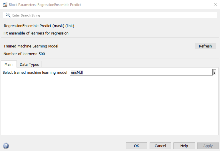
Double-click the RegressionEnsemble Predict block to open the Block Parameters dialog box. Specify the Select trained machine learning model parameter as ensMdl, which is the name of a workspace variable that contains the trained model. Click the Refresh button. The dialog box displays the options used to train the model ensMdl under Trained Machine Learning Model.

The RegressionEnsemble Predict block expects an observation containing 13 predictor values. Double-click the Inport block, and set the Port dimensions to 13 on the Signal Attributes tab.

Create an input signal in the form of a structure array for the Simulink model. The structure array must contain these fields:

time — The points in time at which the observations enter the model. The orientation must correspond to the observations in the predictor data. So, in this example, time must be a column vector.
signals — A 1-by-1 structure array describing the input data and containing the fields values and dimensions, where values is a matrix of predictor data, and dimensions is the number of predictor variables.

Create an appropriate structure array for the slexCarDataRegressionEnsemblePredictExample model from the carsmall data set. When you convert Origin in carsmall to the categorical data type array c_Origin_small, use categories(c_Origin) so that c_Origin and c_Origin_small have the same number of categories in the same order.

load carsmall
c_Origin_small = categorical(cellstr(Origin),categories(c_Origin));
d_Origin_small = dummyvar(c_Origin_small);
testX = [Acceleration,Cylinders,Displacement,Horsepower,Model_Year,Weight,d_Origin_small];
testX = rmmissing(testX);
carsmallInput.time = (0:size(testX,1)-1)';
carsmallInput.signals(1).values = testX;
carsmallInput.signals(1).dimensions = size(testX,2);

To import signal data from the workspace:

Open the Configuration Parameters dialog box. On the Modeling tab, click Model Settings.
In the Data Import/Export pane, select the Input check box and enter carsmallInput in the adjacent text box.
In the Solver pane, under Simulation time, set Stop time to carsmallInput.time(end). Under Solver selection, set Type to Fixed-step, and set Solver to discrete (no continuous states).

For more details, see Load Signal Data for Simulation (Simulink).

Simulate the model.

sim(SimMdlName);

When the Inport block detects an observation, it directs the observation into the RegressionEnsemble Predict block. You can use the Simulation Data Inspector (Simulink) to view the logged data of the Outport block.

Predict Responses Using RegressionEnsemble Predict Block

Train Regression Model with Optimal Hyperparameters

Create Simulink Model

See Also

Related Topics