Regularize Logistic Regression

Step 1. Prepare the data.

Load the ionosphere data. The response Y is a cell array of 'g' or 'b' characters. Convert the cells to logical values, with true representing 'g'. Remove the first two columns of X because they have some awkward statistical properties, which are beyond the scope of this discussion.

load ionosphere
Ybool = strcmp(Y,'g');
X = X(:,3:end);

Step 2. Create a cross-validated fit.

Construct a regularized binomial regression using 25 Lambda values and 10-fold cross validation. This process can take a few minutes.

rng('default') % for reproducibility
[B,FitInfo] = lassoglm(X,Ybool,'binomial',...
    'NumLambda',25,'CV',10);

Step 3. Examine plots to find appropriate regularization.

lassoPlot can give both a standard trace plot and a cross-validated deviance plot. Examine both plots.

lassoPlot(B,FitInfo,'PlotType','CV');
legend('show','Location','best') % show legend

The plot identifies the minimum-deviance point with a green circle and dashed line as a function of the regularization parameter Lambda. The blue circled point has minimum deviance plus no more than one standard deviation.

lassoPlot(B,FitInfo,'PlotType','Lambda','XScale','log');

The trace plot shows nonzero model coefficients as a function of the regularization parameter Lambda. Because there are 32 predictors and a linear model, there are 32 curves. As Lambda increases to the left, lassoglm sets various coefficients to zero, removing them from the model.

The trace plot is somewhat compressed. Zoom in to see more detail.

xlim([.01 .1])
ylim([-3 3])

As Lambda increases toward the left side of the plot, fewer nonzero coefficients remain.

Find the number of nonzero model coefficients at the Lambda value with minimum deviance plus one standard deviation point. The regularized model coefficients are in column FitInfo.Index1SE of the B matrix.

indx = FitInfo.Index1SE;
B0 = B(:,indx);
nonzeros = sum(B0 ~= 0)

nonzeros =

    14

When you set Lambda to FitInfo.Index1SE, lassoglm removes over half of the 32 original predictors.

Step 4. Create a regularized model.

The constant term is in the FitInfo.Index1SE entry of the FitInfo.Intercept vector. Call that value cnst.

The model is logit(mu) = log(mu/(1 - mu)) = X*B0 + cnst. Therefore, for predictions, mu = exp(X*B0 + cnst)/(1+exp(x*B0 + cnst)).

The glmval function evaluates model predictions. It assumes that the first model coefficient relates to the constant term. Therefore, create a coefficient vector with the constant term first.

cnst = FitInfo.Intercept(indx);
B1 = [cnst;B0];

Step 5. Examine residuals.

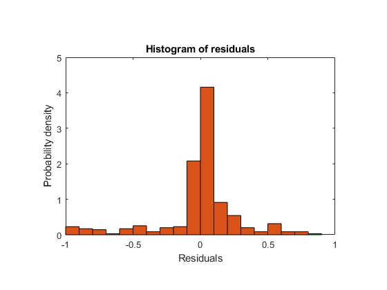
Plot the training data against the model predictions for the regularized lassoglm model.

preds = glmval(B1,X,'logit');
histogram(Ybool - preds) % plot residuals
title('Residuals from lassoglm model')

Step 6. Alternative: Use identified predictors in a least-squares generalized linear model.

Instead of using the biased predictions from the model, you can make an unbiased model using just the identified predictors.

predictors = find(B0); % indices of nonzero predictors
mdl = fitglm(X,Ybool,'linear',...
    'Distribution','binomial','PredictorVars',predictors)

mdl = 


Generalized linear regression model:
    y ~ [Linear formula with 15 terms in 14 predictors]
    Distribution = Binomial

Estimated Coefficients:
                   Estimate       SE        tStat        pValue  
                   _________    _______    ________    __________

    (Intercept)      -2.9367    0.50926     -5.7666    8.0893e-09
    x1                 2.492    0.60795       4.099    4.1502e-05
    x3                2.5501    0.63304      4.0284     5.616e-05
    x4               0.48816    0.50336      0.9698       0.33215
    x5                0.6158    0.62192     0.99015        0.3221
    x6                 2.294     0.5421      4.2317    2.3198e-05
    x7               0.77842    0.57765      1.3476        0.1778
    x12               1.7808    0.54316      3.2786     0.0010432
    x16            -0.070993    0.50515    -0.14054       0.88823
    x20              -2.7767    0.55131     -5.0365    4.7402e-07
    x24               2.0212    0.57639      3.5067    0.00045372
    x25              -2.3796    0.58274     -4.0835    4.4363e-05
    x27              0.79564    0.55904      1.4232       0.15467
    x29               1.2689    0.55468      2.2876      0.022162
    x32              -1.5681    0.54336     -2.8859     0.0039035


351 observations, 336 error degrees of freedom
Dispersion: 1
Chi^2-statistic vs. constant model: 262, p-value = 1e-47

Plot the residuals of the model.

plotResiduals(mdl)

As expected, residuals from the least-squares model are slightly smaller than those of the regularized model. However, this does not mean that mdl is a better predictor for new data.