Regularize Wide Data in Parallel

This example shows how to regularize a model with many more predictors than observations. Wide data is data with more predictors than observations. Typically, with wide data you want to identify important predictors. Use lassoglm as an exploratory or screening tool to select a smaller set of variables to prioritize your modeling and research. Use parallel computing to speed up cross validation.

Load the ovariancancer data. This data has 216 observations and 4000 predictors in the obs workspace variable. The responses are binary, either 'Cancer' or 'Normal', in the grp workspace variable. Convert the responses to binary for use in lassoglm.

load ovariancancer
y = strcmp(grp,'Cancer');

Set options to use parallel computing. Prepare to compute in parallel using parpool.

opt = statset('UseParallel',true);
parpool()

Starting parallel pool (parpool) using the 'local' profile ...
Connected to the parallel pool (number of workers: 6).

ans = 

 ProcessPool with properties: 

            Connected: true
           NumWorkers: 6
              Cluster: local
        AttachedFiles: {}
    AutoAddClientPath: true
          IdleTimeout: 30 minutes (30 minutes remaining)
          SpmdEnabled: true

Fit a cross-validated set of regularized models. Use the Alpha parameter to favor retaining groups of highly correlated predictors, as opposed to eliminating all but one member of the group. Commonly, you use a relatively large value of Alpha.

rng('default') % For reproducibility
tic
[B,S] = lassoglm(obs,y,'binomial','NumLambda',100, ...
  'Alpha',0.9,'LambdaRatio',1e-4,'CV',10,'Options',opt);
toc

Elapsed time is 90.892114 seconds.

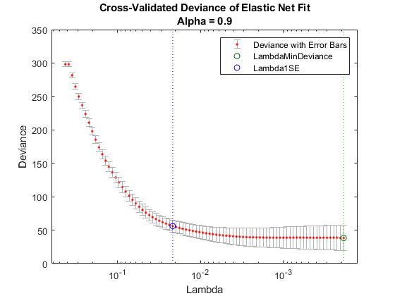
Examine cross-validation plot.

lassoPlot(B,S,'PlotType','CV');     
legend('show') % Show legend

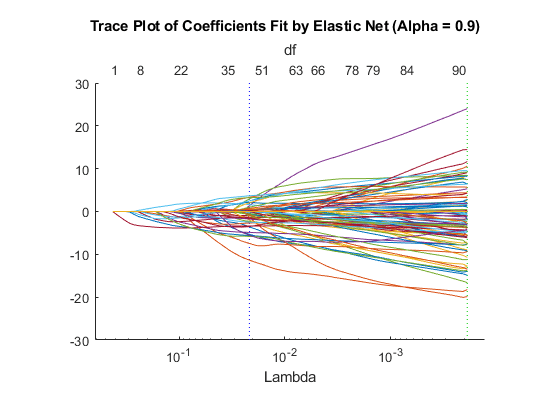
Examine trace plot.

lassoPlot(B,S,'PlotType','Lambda','XScale','log')

The right (green) vertical dashed line represents the Lambda providing the smallest cross-validated deviance. The left (blue) dashed line has the minimal deviance plus no more than one standard deviation. This blue line has many fewer predictors:

[S.DF(S.Index1SE) S.DF(S.IndexMinDeviance)]

ans = 1×2

    50    89

You asked lassoglm to fit using 100 different Lambda values. How many did it use?

size(B)

ans = 1×2

        4000          84

lassoglm stopped after 84 values because the deviance was too small for small Lambda values. To avoid overfitting, lassoglm halts when the deviance of the fitted model is too small compared to the deviance in the binary responses, ignoring the predictor variables.

You can force lassoglm to include more terms by using the 'Lambda' name-value pair argument. For example, define a set of Lambda values that additionally includes three values smaller than the values in S.Lambda.

minLambda = min(S.Lambda);
explicitLambda = [minLambda*[.1 .01 .001] S.Lambda];

Specify 'Lambda',explicitLambda when you call the lassoglm function. lassoglm halts when the deviance of the fitted model is too small, even though you explicitly provide a set of Lambda values.

To save time, you can use:

Use serial computation and all three of these time-saving methods:

tic
[Bquick,Squick] = lassoglm(obs,y,'binomial','NumLambda',25,...
    'LambdaRatio',1e-2,'CV',5);
toc

Elapsed time is 16.517331 seconds.

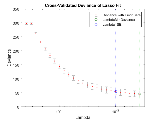
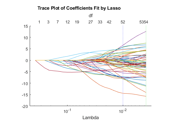
Graphically compare the new results to the first results.

lassoPlot(Bquick,Squick,'PlotType','CV');     
legend('show') % Show legend

lassoPlot(Bquick,Squick,'PlotType','Lambda','XScale','log')

The number of nonzero coefficients in the lowest plus one standard deviation model is around 50, similar to the first computation.