Maxima, Minima, and Inflection Points

First Derivatives: Finding Local Minima and Maxima

Computing the first derivative of an expression helps you find local minima and maxima of that expression. For example, create a rational expression where the numerator and the denominator are polynomial expressions.

syms x
f = (3 * x^3 + 17 * x^2 + 6 * x + 1)/(2 * x^3 + x * -1 + 3)

f = 
$$\frac{3\hspace{0.17em}{x}^3+17\hspace{0.17em}{x}^2+6\hspace{0.17em}x+1}{2\hspace{0.17em}{x}^3-x+3}$$

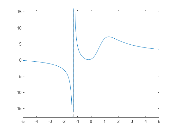
Plotting this expression shows that it has horizontal and vertical asymptotes, a local minimum between -1 and 0, and a local maximum between 1 and 2.

fplot(f)

By default, when you operate on this expression, results can include both real and imaginary numbers. If you are interested in real numbers only, you can set the permanent assumption that x belongs to the set of real numbers. This allows you to avoid complex numbers in the solutions and it also can improve performance.

assume(x, 'real')

To find a horizontal asymptote, compute the limit of $$f$$ for x approaching positive and negative infinities. The horizontal asymptote is $$x=3/2$$.

[limit(f, x, sym(inf)), limit(f, x, -sym(inf))]

ans = 
$$\left(\begin{array}{cc}\frac{3}{2}& \frac{3}{2}\end{array}\right)$$

To find a vertical asymptote of $$f$$, find the roots of the polynomial expression that represents the denominator of $$f$$.

solve(2 * x^3 + x * -1 + 3 == sym(0), x)

ans = 
$$\mathrm{root}\left(z^3-\frac{z}{2}+\frac{3}{2},z,3\right)$$

To get an explicit solution for such equations, try calling the solver with the option MaxDegree. The option specifies the maximum degree of polynomials for which the solver tries to return explicit solutions. By default, MaxDegree = 2. Increasing this value, you can get explicit solutions for higher-order polynomials. For example, specifying MaxDegree = 3 results in an explicit solution.

solve(2 * x^3 + x * -1 + 3 == 0, x, 'MaxDegree', 3)

ans = 
$$-\frac{1}{6\hspace{0.17em}{\left(\frac{3}{4}-\frac{\sqrt{241}\hspace{0.17em}\sqrt{432}}{432}\right)}^{1/3}}-{\left(\frac{3}{4}-\frac{\sqrt{241}\hspace{0.17em}\sqrt{432}}{432}\right)}^{1/3}$$

You can approximate the exact solution numerically by using the vpa function.

vpa(ans,6)

ans = $$-1.28962$$

Now find the local minimum and maximum of the expression f. If the point is a local extremum (either minimum or maximum), the first derivative of the expression at that point is equal to zero. To compute the derivative of an expression, use the diff function.

g = diff(f, x)

g = 
$$\frac{9\hspace{0.17em}{x}^2+34\hspace{0.17em}x+6}{2\hspace{0.17em}{x}^3-x+3}-\frac{\left(6\hspace{0.17em}{x}^2-1\right)\hspace{0.17em}\left(3\hspace{0.17em}{x}^3+17\hspace{0.17em}{x}^2+6\hspace{0.17em}x+1\right)}{{\left(2\hspace{0.17em}{x}^3-x+3\right)}^2}$$

To find the local extrema of f, solve the equation g = 0. If you use the MaxDegree option, the solver returns the long explicit solution, which can be approximated by using the vpa function.

solve(g == 0, x, 'MaxDegree', 4);
extrema = vpa(ans, 6)

extrema = 
$$\left(\begin{array}{c}-0.189245\\ 1.28598\end{array}\right)$$

The plot of the expression f shows that x = -0.189 is a local minimum of the expression, and x = 1.286 is its local maximum.

fplot(f)
hold on
plot(extrema, subs(f,extrema), '*')
hold off

Second Derivatives: Finding Inflection Points

Computing the second derivative lets you find inflection points of the expression.

h(x) = simplify(diff(f, x, 2))

h(x) = 
$$\frac{2\hspace{0.17em}\left(68\hspace{0.17em}{x}^6+90\hspace{0.17em}{x}^5+18\hspace{0.17em}{x}^4-699\hspace{0.17em}{x}^3-249\hspace{0.17em}{x}^2+63\hspace{0.17em}x+172\right)}{{\left(2\hspace{0.17em}{x}^3-x+3\right)}^3}$$

To find inflection points of $$f$$, solve the equation h = 0. For this equation the symbolic solver returns a complicated result even if you use the MaxDegree option.

solve(h == 0, x, 'MaxDegree', 4)

ans = 
$$\begin{array}{l}\left(\begin{array}{c}\mathrm{root}\left({\sigma }_1,z,1\right)\\ \mathrm{root}\left({\sigma }_1,z,4\right)\end{array}\right)\\ \\ \mathrm{where}\\ \\ \mathrm{ }{\sigma }_1=z^6+\frac{45\hspace{0.17em}{z}^5}{34}+\frac{9\hspace{0.17em}{z}^4}{34}-\frac{699\hspace{0.17em}{z}^3}{68}-\frac{249\hspace{0.17em}{z}^2}{68}+\frac{63\hspace{0.17em}z}{68}+\frac{43}{17}\end{array}$$

To get the simpler numerical result, solve the equation numerically by using vpasolve; specify the search range to restrict the returned results to all real solutions of the expression.

inflection = vpasolve(h == 0, x, [-inf, inf])

inflection = 
$$\left(\begin{array}{c}0.57871842655441748319601085860196\\ 1.8651543689917122385037075917613\end{array}\right)$$

The expression f has two inflection points: x = 0.579 and x = 1.865.

fplot(f)
hold on
plot(extrema, subs(f,extrema), '*')
plot(inflection, subs(f,inflection), '*')
hold off

Suprema

Not all functions can be treated analytically; the function

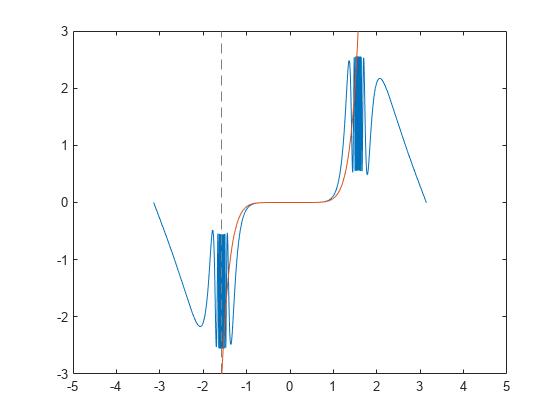
is very flat at the origin and it oscillates infinitely often near $$-\frac{\pi }{2}$$, becomes linear as it approaches zero and oscillates again near $$\pi$$.

f = @(x) tan(sin(x))-sin(tan(x))

f = function_handle with value:
    @(x)tan(sin(x))-sin(tan(x))

fplot(f, [-pi , pi])

Most important for our purposes here, fplot has picked the limit on the y-axes to be

ylim

ans = 1×2

   -2.5488    2.5572

What is happening at $$\frac{\pi }{2}$$?

MATLAB® uses double precision arithmetic, so $$\frac{\pi }{2}$$ evaluates to one of the oscillations.

pi/2

ans = 
1.5708

f(pi/2)

ans = 
2.5161

The Symbolic Math Toolbox uses exact arithmetic, which shows the function is undefined.

syms x
sym(pi/2)

ans = 
$$\frac{\pi }{2}$$

F = sym(f)

F = $$\tan \left(\sin \left(x\right)\right)-\sin \left(\tan \left(x\right)\right)$$

subs(F,x,sym(pi/2))

ans = $$\mathrm{NaN}$$

Taylor Series

We can also try to look at the value with a Taylor Series.

T = taylor(F,x,'Order',10,'ExpansionPoint',0)

T = 
$$\frac{29\hspace{0.17em}{x}^9}{756}+\frac{x^7}{30}$$

vpa(subs(T,x,pi/2))

ans = $$3.0198759869735883213825972535797$$

hold on 
fplot(T)
ylim ([-3 3])
hold off

Calculus

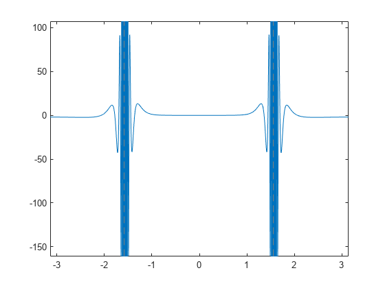
We learn in calculus that a maximum occurs at a zero of the derivative. But this function is not differentiable in the vicinity of $$\frac{\pi }{2}$$. We can analytically differentiate $$f(x)$$ using the Symbolic Math Toolbox.

diff(F)

ans = $$\cos \left(x\right)\hspace{0.17em}\left({\tan \left(\sin \left(x\right)\right)}^2+1\right)-\cos \left(\tan \left(x\right)\right)\hspace{0.17em}\left({\tan \left(x\right)}^2+1\right)$$

fplot(diff(F), [-pi , pi])

Sampling

We can sample the function N times near $$\frac{\pi }{2}$$ to get a numerical approximation to the value of the maximum. Is that good enough?

N = 100;
xValues = 3*pi/8 + pi/4*rand(1,N) 

xValues = 1×100

    1.8180    1.8895    1.2778    1.8955    1.6748    1.2547    1.3968    1.6076    1.9301    1.9359    1.3019    1.9404    1.9299    1.5593    1.8066    1.2895    1.5093    1.8973    1.8003    1.9317    1.6931    1.2061    1.8450    1.9117    1.7112    1.7732    1.7618    1.4862    1.6929    1.3125    1.7326    1.2031    1.3956    1.2144    1.2544    1.8248    1.7238    1.4271    1.9244    1.2052    1.5227    1.4778    1.7793    1.8026    1.3249    1.5628    1.5281    1.6857    1.7352    1.7708

ySoln = f(xValues)

ySoln = 1×100

    0.7260    1.5080    1.5932    1.5614    1.3796    1.3158    2.0658    2.4586    1.8194    1.8541    1.9088    1.8793    1.8178    2.3439    0.6145    1.7447    2.0697    1.5775    0.5629    1.8290    2.4930    0.8543    1.0347    1.6931    2.2371    0.5024    0.6011    2.2489    2.4891    2.0499    1.3564    0.8308    2.0986    0.9208    1.3122    0.8011    1.7177    0.9333    1.7830    0.8466    0.6138    2.5047    0.4857    0.5809    2.2051    2.5133    2.5387    2.2247    1.2583    0.5153

max(ySoln)

ans = 
2.5387

Proof

Determine the maximum from a mathematical proof.

so $$\sin (\tan (x))\le 1$$ and $$tan(sin(x))\le \tan (1)$$ which means consequently

As $$x\Rightarrow \frac{\pi }{2}$$, $$\tan (x)$$ oscillates and blows up; so$$f(x)$$ is actually not defined at all at this point as was shown above

Now we can take a look at the numerical value.

format long 
1 + tan(1) 

ans = 
   2.557407724654902