Next Step Suggestions for Symbolic Workflows in Live Editor
Starting in R2021b, when you run code that generates a symbolic output in the Live Editor, Live Editor provides a context menu with next step suggestions that are specific to the output. To open the suggestion menu, you can point your mouse to the symbolic output and click the three-dot icon ![]() , or you can right-click the symbolic output. When reopening your symbolic workflow live script, run the code again to get the next step suggestions.
, or you can right-click the symbolic output. When reopening your symbolic workflow live script, run the code again to get the next step suggestions.
Starting in R2023b, you can also use keyboard shortcuts to navigate to the next step suggestions after you run your code. To move between code and output in the Live Editor, use the Up/Down Arrow when the output is inline, or use Ctrl+Shift+O (on macOS systems, use Option+Command+O instead) when the output is on the right. Activate the symbolic output by pressing the Return key. Use the shortcut Shift+F10 to open the suggestion menus.
Using these suggestion menus, you can insert and execute function calls or Live Editor tasks into live scripts. Typical uses of these suggestion menus include:
Evaluate and convert symbolic expressions to numeric values.
Simplify and manipulate, or solve symbolic math equations.
Plot symbolic expressions.
Perform matrix and vector operations, such as finding the inverse and determinant of a matrix, and finding the Jacobian and curl of a vector.
Perform calculus functions, such as differentiation, integration, transforms, and solving differential equations.
Convert between units of measurement and verify unit dimensions.
For example, in a new live script, create a symbolic expression.
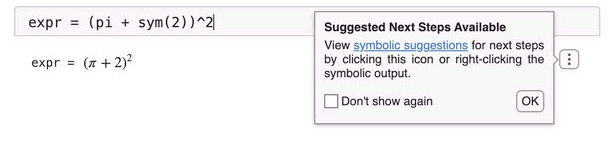
expr = (pi + sym(2))^2
expr =
Click Run to see the result, which is a symbolic output. When you first run code that generates a symbolic output, Live Editor shows the three-dot icon ![]() for suggested next steps with a pop-up notification. You can also point to the symbolic output to bring up the three-dot icon. To suppress the pop-up notification in the rest of your workflow, select Don't show again.
for suggested next steps with a pop-up notification. You can also point to the symbolic output to bring up the three-dot icon. To suppress the pop-up notification in the rest of your workflow, select Don't show again.
Click the three-dot icon ![]() located to the right of the output to bring up the suggestion menu. When you point to a menu item, Live Editor gives you a preview of what happens when you select the menu item. For instance, if you point to Approximate numerically, you see the new line of code it suggests.
located to the right of the output to bring up the suggestion menu. When you point to a menu item, Live Editor gives you a preview of what happens when you select the menu item. For instance, if you point to Approximate numerically, you see the new line of code it suggests.
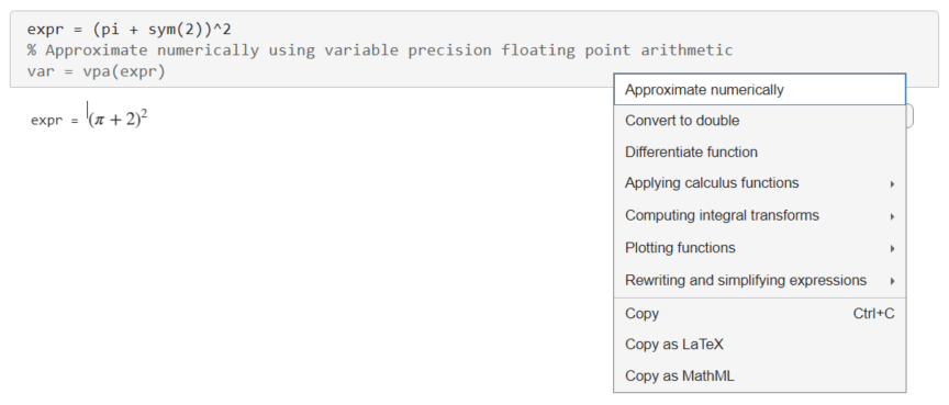
Select Approximate numerically to add the suggested new line of code. Live Editor inserts the vpa function into the code region and automatically runs the current section to evaluate the expression numerically.
var = vpa(expr)
var =
As another example, create a symbolic equation. Run a live script to generate the symbolic output. Solve the equation numerically using symbolic suggestions for next steps.
syms x a
eqn = (2*x^2 + a)/(x + 1) == 3
eqn =
To open the suggestion menu, you can also right-click the symbolic output. Select Solving equations > Solve equation numerically.
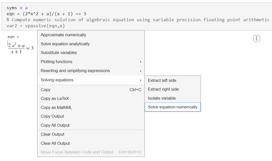
When you click the Solve equation numerically suggestion, Live Editor inserts the vpasolve function into the code region. Live Editor then automatically runs the current section to solve the equation numerically.
var2 = vpasolve(eqn,x)
var2 =
The following sections provide more examples showing how to use the interactive suggestion menus in symbolic workflows.
Simplify Symbolic Expression
Create a symbolic expression that contains exponential functions and imaginary numbers. Run the following code to generate the symbolic output.
syms x
expr = 1i*(exp(-1i*x) - exp(1i*x))/(exp(-1i*x) + exp(1i*x))
expr =
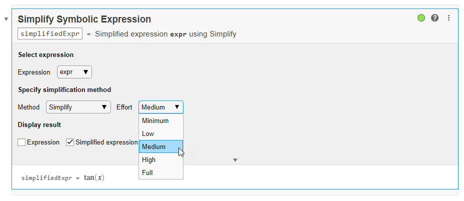
To simplify the expression, right-click the symbolic output and select Rewriting and simplifying expressions > Simplify expression.
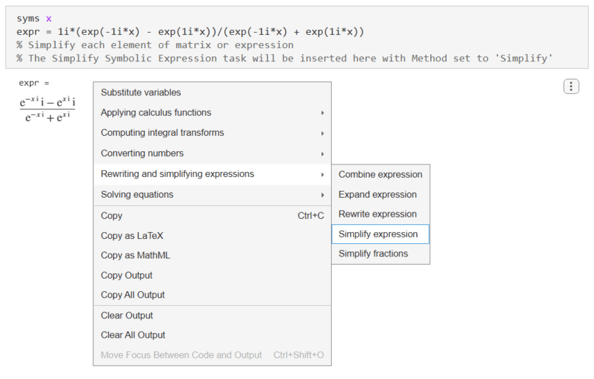
Live Editor inserts and applies the Simplify Symbolic Expression task to interactively simplify or rearrange symbolic expressions. Change the computational effort to Medium to get a simpler result.
Substitute Coefficients and Solve Quadratic Equation
Create a quadratic equation with coefficients , , and . Run the following code to generate the symbolic output.
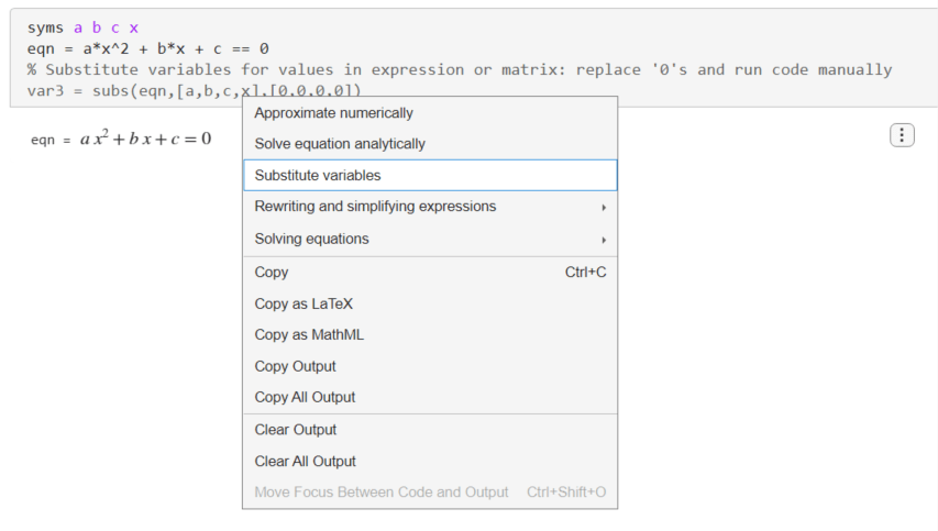
syms a b c x
eqn = a*x^2 + b*x + c == 0
eqn =
To substitute the coefficients in the equation, right-click the output and select Substitute variables.
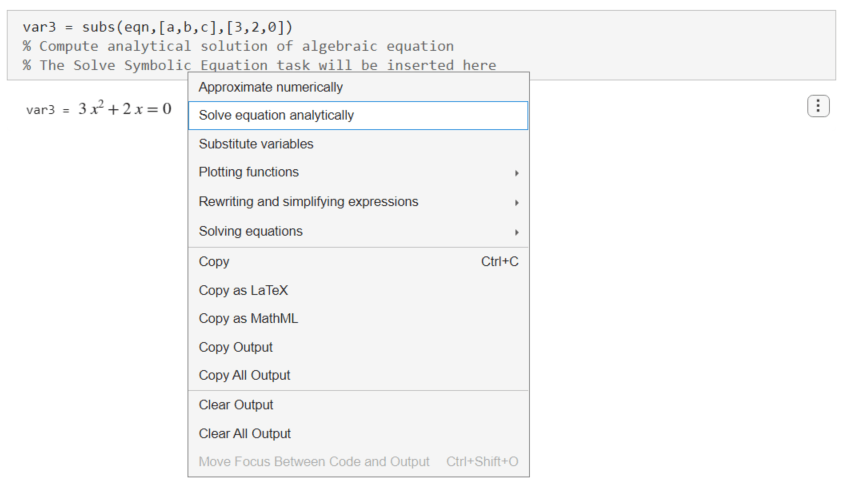
Live Editor inserts the subs function to substitute the coefficients and variables in the equations. For the subs function, Live Editor does not run the function automatically. To substitute , , and , change the second and third arguments of the subs function to [a,b,c] and [3,2,0]. Run the Live Editor section afterward to apply the subs function.
var3 = subs(eqn,[a,b,c],[3,2,0])
var3 =
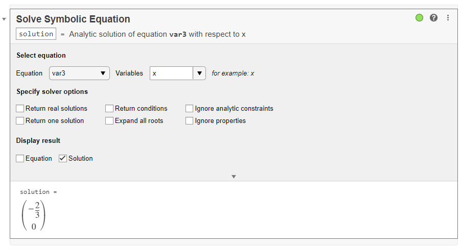
To solve the quadratic equation, right-click the output and select Solve equation analytically.
Live Editor inserts and applies the Solve Symbolic Equation task to interactively find analytic solutions of symbolic equations.
Plot Explicit and Implicit Functions
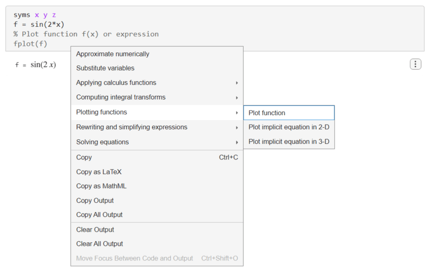
Create three symbolic variables x, y, and z and a sinusoidal function. Run the following code to generate the symbolic output.
syms x y z
f = sin(2*x)
f =
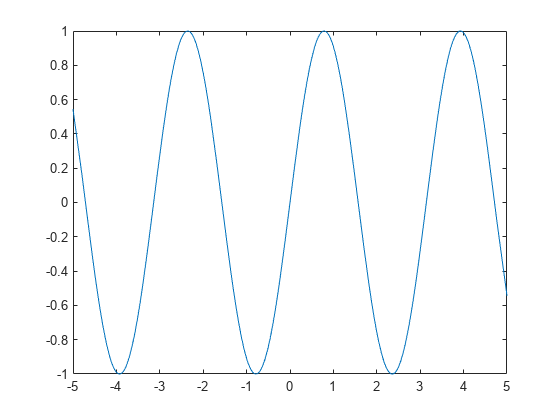
To plot the sinusoidal function, right-click the output and select Plotting functions > Plot function.
Live Editor plots the sinusoidal function using fplot.
fplot(f)
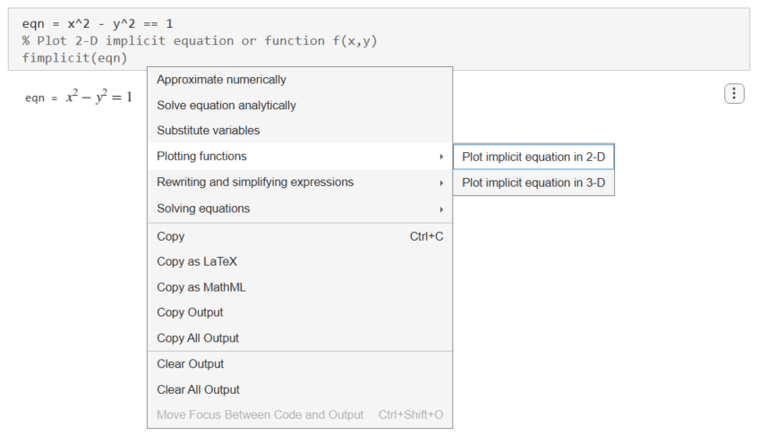
Next, create an equation that represents a hyperbola. Run the following code to generate the symbolic output.
eqn = x^2 - y^2 == 1
eqn =
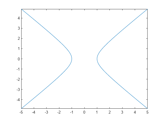
To plot the sinusoidal function, right-click the output and select Plotting functions > Plot implicit equation in 2-D.
Live Editor plots the hyperbola using fimplicit.
fimplicit(eqn)
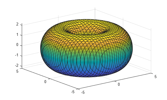
Next, create a symbolic function that represents a torus. Run the following code to generate the symbolic output.
f(x,y,z) = (x^2 + y^2 + z^2 + 3^2 - 2^2)^2 - 4*3^2*(x^2+y^2)
f(x, y, z) =
To plot the torus, right-click the output and select Plot implicit equation in 3-D.
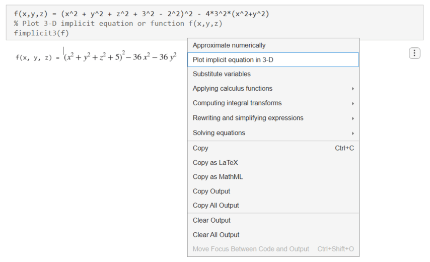
Live Editor plots the torus using fimplicit3.
fimplicit3(f)
Apply Matrix Functions
Create three symbolic variables x, y, and z and a symbolic matrix. Run the following code to generate the symbolic output.
syms x y z
M1 = sym([x^2 + a, x; y + 2, 3*y^2])
M1 =
To invert the matrix, right-click the output and select Applying matrix functions > Invert matrix. Note that the Applying matrix functions > Invert matrix suggestion is available only if the symbolic output is a symbolic matrix.
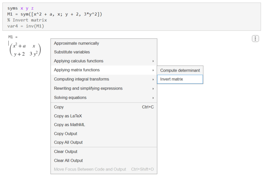
Live Editor inserts and applies the inv function to invert the matrix.
var4 = inv(M1)
var4 =
Next, create a 1-by-3 symbolic vector. Run the following code to generate the symbolic output.
M2 = sym([x*y*z, y^2, x + z])
M2 =
To compute the Jacobian of the vector, right-click the output and select Applying matrix functions > Compute Jacobian matrix of vector. Note that the Applying matrix functions > Compute Jacobian matrix of vector suggestion is available only if the symbolic output is a symbolic vector.
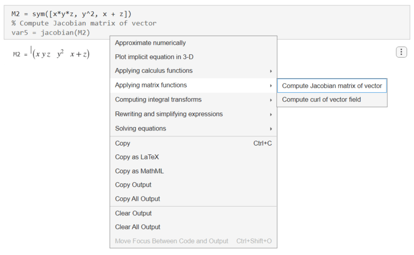
Live Editor inserts and applies the jacobian function to compute the Jacobian of the vector.
var5 = jacobian(M2)
var5 =
Next, create another 1-by-3 symbolic vector. Run the following code to generate the symbolic output.
M3 = sym([x^2*y, 2*x, z])
M3 =
To compute the curl of the vector, right-click the output and select Applying matrix functions > Compute curl of vector field.
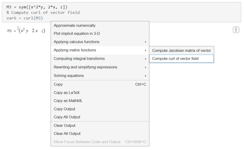
Live Editor inserts and applies the curl function to compute the curl of the vector.
var6 = curl(M3)
var6 =
Solve Differential Equation, Compute Integral Transform, and Find Poles
Create a second-order differential equation. Run the following code to generate the symbolic output.
syms f(x) s
eqn = diff(f,x,x) == -9*f
eqn(x) =
To solve the differential equation, right-click the output and select Solve differential equation. Note that the Solve differential equation suggestion is available only if the symbolic output is a differential equation.
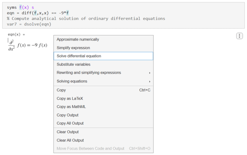
Live Editor inserts and applies the dsolve function to solve the differential equation.
var7 = dsolve(eqn)
var7 =
Next, find the Laplace transform of the solution. Right-click the output of dsolve and select Computing integral transforms > Compute Laplace transform.
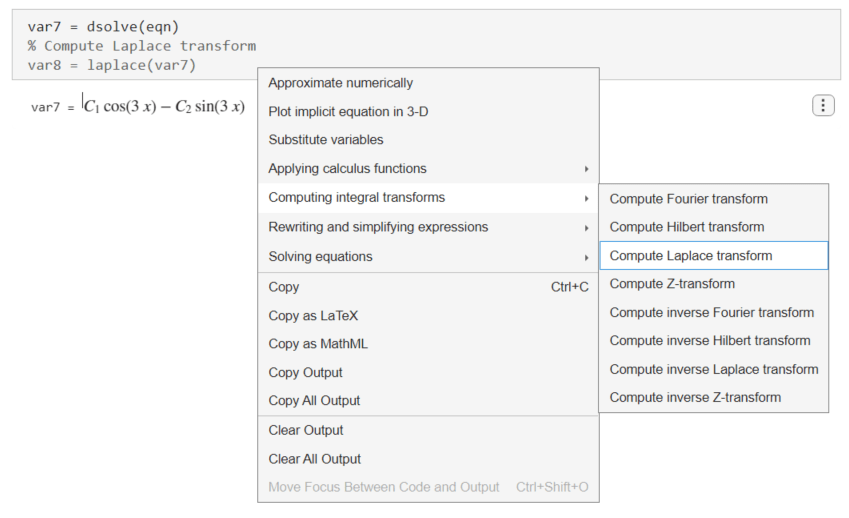
Live Editor inserts and applies the laplace function to compute the Laplace transform.
var8 = laplace(var7)
var8 =
Finally, find the poles of the Laplace transform. Right-click the output of the Laplace transform and select Applying calculus functions > Compute poles of function.
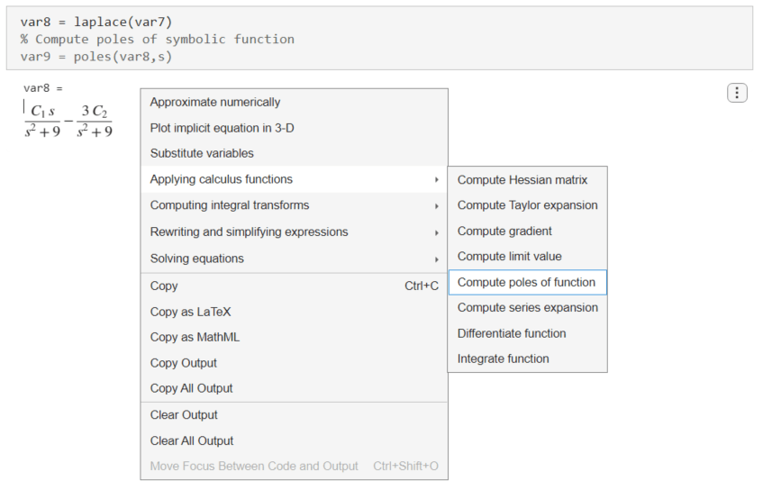
Live Editor inserts and applies the poles function to compute the poles.
var9 = poles(var8,s)
var9 =
Convert Units and Check Consistency of Units
Create a ratio of two lengths with different units. Run the following code to generate the symbolic output.
u = symunit;
ratio = (7*u.mi)/(420*u.ft)
ratio =
Convert the units to the meter-gram-second system. Right-click the output and select Applying physical unit functions > Convert units. Note that the Applying physical unit functions suggestion is available only if the symbolic output contains symbolic units.
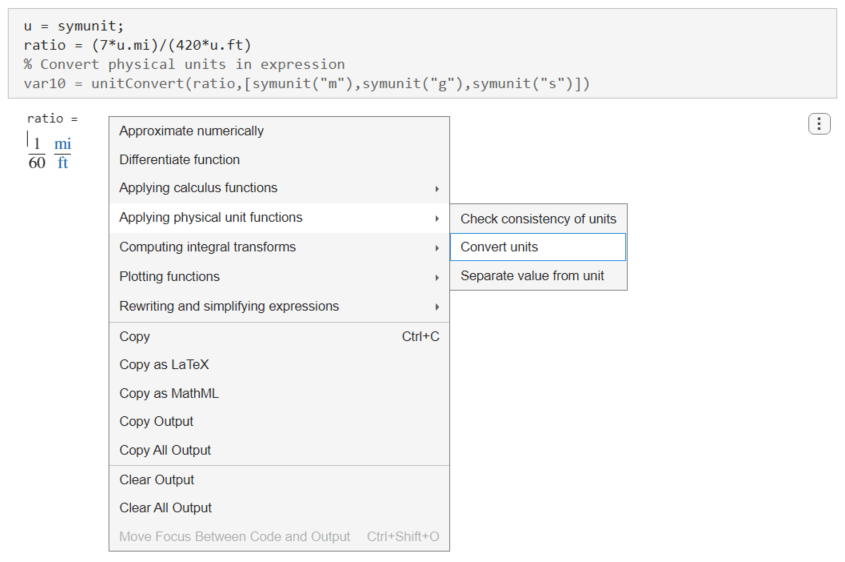
Live Editor inserts and applies the unitConvert function to convert the units to the meter-gram-second system.
var10 = unitConvert(ratio,[symunit('m'),symunit('g'),symunit('s')])
var10 =
Next, create two symbolic expressions x and y that describe the - and -coordinates of a moving projectile. Create a symbolic equation r that compares the units of x and y to the length units m and ft. Run the following code to generate the symbolic output.
syms theta ts x y r
g = 9.81*u.m/u.s^2;
v = 10*u.m/u.s;
t = ts*u.s;
x = v*cos(theta)*t;
y = v*sin(theta)*t + (-g*t^2)/2;
r = [x == u.m y == u.ft]
r =
Check the consistency of units in r. Right-click the output and select Applying physical unit functions > Check consistency of units.
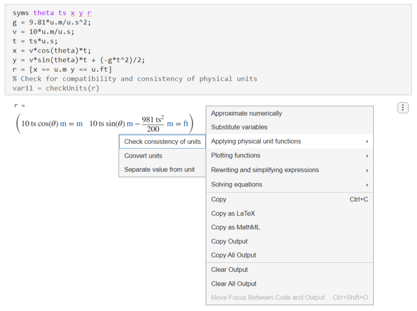
Live Editor inserts and applies the checkUnits function to check the consistency and compatibility of the units in r.
The checkUnits function returns a structure containing the fields Consistent and Compatible. The Consistent field returns logical 1(true) if all terms in r have the same dimension and same unit with a conversion factor of 1. The Compatible field returns logical 1(true) if all terms have the same dimension, but not necessarily the same unit.
var11 = checkUnits(r)
var11 = struct with fields:
    Consistent: [1 0]
    Compatible: [1 1]