Adapt Image Filter Coefficients from Frame to Frame

The Example Model

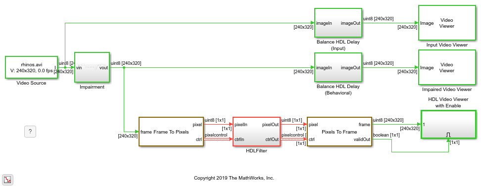
The example model applies a brightness impairment to the input video, and the HDL Filter subsystem calculates filter coefficients for each frame and corrects the impairment. The model includes three video viewers: one for the original input video, another for the impaired video, and the third for the result of the filter that counteracts the impairment.

The model also includes Frame to Pixels and Pixels to Frame blocks to convert the matrix format video to streaming format suitable for HDL modeling.

The Impairment

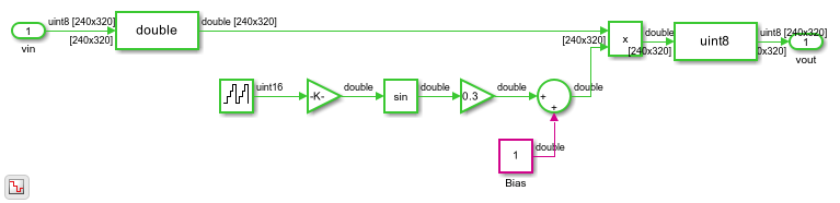
The impairment in this model is brightness modulation using a slow sine wave. Since the impairment is modeled purely behaviorally, the first step is to convert the image to double-precision values. The 16-bit counter counts up at the frame rate and the counter value is multiplied by 2*pi/40. The sine wave output is scaled down by 0.3 and a bias of 1.0 is then added. These calculations result in a +/-30% change in brightness over a period of 40 frames. After applying the impairment, the model converts back to uint8 by using rounding with saturation.

The Filter Algorithm

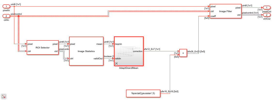
The HDL Algorithm subsystem starts by extracting a region of interest in the center of the image. Since this model is configured for a 320x240 video source, it uses a 100x100 region in the center of the video stream.

The Image Statistics block finds the mean of that central region. A new mean is computed for each 100x100 frame. The block sets the validOut port to true to indicate when the new mean is valid.

Compute the Scaled Grand Mean

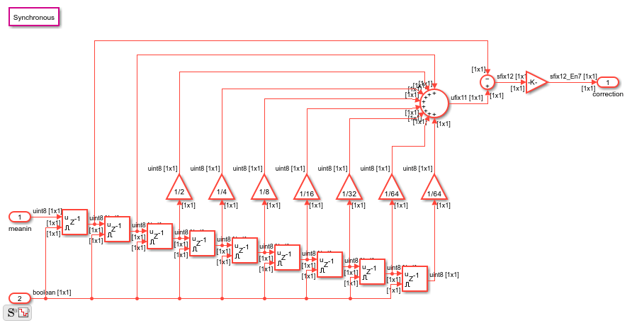
The Adapt Grand Mean subsystem computes the correction factor required to counteract the impairment.

You could use central-region-mean brightness directly, with a "gray-world" assumption that the average brightness is mid-scale (128 in this case). But, a more accurate approach is to use the previous brightness means, with the assumption that the average brightness does not change quickly frame to frame.

Forming a mean of means is known as a grand mean, but that calculation would give equal weight to the past frames. Instead, the subsystem weights the past frames with an exponential fractional decay with the coefficients [1 1/2 1/4 1/8 1/16 1/32 1/64 1/64]. The last coefficient would normally be 1/128 but by adjusting that value, the sum of the weights becomes exactly 2, making the normalizing factor a simple shift operation. Note that the initial value of all the delay line registers is mid-scale (128) to avoid large start-up transients in the correction.

The subsystem finds the correction factor using the current mean and the weighted grand mean. Since the grand mean scaled up by 2, if you subtract the current mean from it, the resulting value is the weighted grand mean plus or minus the error term in the direction of correcting the error.

The correction is then scaled by 2^-7 and sent to the output port. A normalization could be applied here by dividing by the grand mean, but in practice, simple scaling works well enough.

Apply the Correction

The correction output from the Adapt Grand Mean subsystem is then used to scale the filter coefficients, in this case a Gaussian filter of size 5x5 with a standard deviation of the default 0.5. In the actual FPGA this filter uses 25 multipliers. Pipelining is of no concern here since these values are computed well before they are needed. The block samples the coefficient port when the vStart signal in the input ctrl bus is true.

Going Further

In this simple example, you could alternatively apply the correction factor to the scalar pixel stream and then filter. The architecture shown can expand for more complex adaptive changes in the filter coefficients.

The 5x5 multiply of the correction factor with the gaussian coefficients could be implemented as a single serial multiplier rather than 25 parallel multipliers. To achieve this HDL implementation, include the Product block in a Subsystem, and right-click the Subsystem to open the HDL Block Properties. Set the SharingFactor property to 25 to implement a single time-multiplexed multiplier. With this setting, the multiply operation uses a 25-times faster clock than the rest of the design. Consider your required pixel clock speed and whether your device can accommodate the faster rate.