标定 XCP 特征变量
此示例说明如何使用 XCP 协议功能连接和标定来自 XCP Sample 服务器的可用特征变量数据。XCP Sample 服务器是专门为 XCP 示例设计的。
Vehicle Network Toolbox™ 提供 MATLAB® 函数,用于通过多个传输层与服务器对接,包括控制器局域网 (CAN)、控制器局域网灵活数据速率 (CAN FD)、传输控制协议 (TCP) 和用户数据报协议 (UDP)。此示例执行写入以标定参数,然后比较标定前后的测量变量值。
XCP 是一种高级协议,用于访问和修改模型、算法或 ECU 的内部参数和变量。有关详细信息,请参阅 ASAM 标准。
打开 A2L 文件
建立与 XCP 服务器的连接需要 A2L 文件。A2L 文件说明 XCP 服务器提供的所有功能,以及如何连接到该服务器的详细信息。使用 xcpA2L 函数打开说明服务器模型的 A2L 文件。
a2lInfo = xcpA2L("SampleECU.a2l")a2lInfo =
A2L with properties:
File Details
FileName: 'SampleECU.a2l'
FilePath: '/tmp/Bdoc26a_3233028_2243768/tp6061b4c6/vnt-ex60761655/SampleECU.a2l'
ServerName: 'SampleServer'
Warnings: [0×0 string]
Parameter Details
Events: {'Event DAQ 100ms'}
EventInfo: [1×1 xcp.a2l.Event]
Measurements: {'Line' 'PWM' 'Sine'}
MeasurementInfo: [3×1 containers.Map]
Characteristics: {'Gain' 'yData'}
CharacteristicInfo: [2×1 containers.Map]
AxisInfo: [1×1 containers.Map]
RecordLayouts: [3×1 containers.Map]
CompuMethods: [1×1 containers.Map]
CompuTabs: [0×1 containers.Map]
CompuVTabs: [0×1 containers.Map]
XCP Protocol Details
ProtocolLayerInfo: [1×1 xcp.a2l.ProtocolLayer]
DAQInfo: [1×1 xcp.a2l.DAQ]
TransportLayerCANInfo: [1×1 xcp.a2l.XCPonCAN]
TransportLayerUDPInfo: [0×0 xcp.a2l.XCPonIP]
TransportLayerTCPInfo: [1×1 xcp.a2l.XCPonIP]
启动 XCP Sample 服务器
XCP Sample 服务器以可控方式模拟真实 XCP 服务器的行为。在这种情况下,它仅用于演示功能有限的示例。使用本地 SampleECU 类创建 Sample 服务器对象,Sample 服务器将在 MATLAB 工作区中创建。XCP Sample 服务器支持 CAN、CAN FD 和 TCP。此示例选择 CAN 协议进行演示。
sampleServer = SampleECU(a2lInfo,"CAN","MathWorks","Virtual 1",1);
创建 XCP 通道
要创建到服务器的活动 XCP 连接,请使用 xcpChannel 函数。该函数需要引用服务器 A2L 文件以及用于与服务器进行报文传输的传输协议类型。XCP 通道必须使用与 Sample 服务器相同的设备和 a2l 文件,以确保它们可以连接。
xcpCh = xcpChannel(a2lInfo,"CAN","MathWorks","Virtual 1",1)
xcpCh =
  Channel with properties:

              ServerName: 'SampleServer'
             A2LFileName: 'SampleECU.a2l'
          TransportLayer: 'CAN'
    TransportLayerDevice: [1×1 struct]
              SeedKeyDLL: []
             ConnectMode: 'normal'
连接到服务器
要激活与服务器的通信,请使用 connect 函数。
connect(xcpCh);
从 A2L 文件查看可用特征变量
XCP 的特征变量表示模型内存中的可调参数。可用于标定的特征变量在 A2L 文件中定义,可在 Characteristics 属性中找到。请注意,参数 Gain 是乘数,yData 指定一维查找表的输出数据点。
a2lInfo.Characteristics
ans = 1×2 cell
    {'Gain'}    {'yData'}
a2lInfo.CharacteristicInfo("Gain")ans =
Characteristic with properties:
Name: 'Gain'
LongIdentifier: 'Scalar SBYTE'
CharacteristicType: VALUE
ECUAddress: 8454145
Deposit: [1×1 xcp.a2l.RecordLayout]
MaxDiff: 0
Conversion: [1×1 xcp.a2l.CompuMethod]
LowerLimit: -100
UpperLimit: 100
Dimension: 1
AxisConversion: {1×0 cell}
BitMask: []
ByteOrder: MSB_LAST
Discrete: []
ECUAddressExtension: 0
Format: '%6.1'
Number: []
PhysUnit: ''
a2lInfo.CharacteristicInfo("yData")ans =
Characteristic with properties:
Name: 'yData'
LongIdentifier: 'Curve with standard axis'
CharacteristicType: CURVE
ECUAddress: 8454912
Deposit: [1×1 xcp.a2l.RecordLayout]
MaxDiff: 0
Conversion: [1×1 xcp.a2l.CompuMethod]
LowerLimit: 0
UpperLimit: 255
Dimension: 8
AxisConversion: {[1×1 xcp.a2l.CompuMethod]}
BitMask: []
ByteOrder: MSB_LAST
Discrete: []
ECUAddressExtension: 0
Format: ''
Number: []
PhysUnit: ''
标定特征变量增益值
特征变量 Gain 用于计算测量变量 Sine 的值。Gain 的值用于控制测量变量 Sine 的振幅。
检查预加载的特征变量值
读取特征变量 Gain 的当前值。readCharacteristic 函数对给定的特征变量执行从服务器的直接读取。
initialGain = readCharacteristic(xcpCh, "Gain")initialGain = 2
获取标定前的测量变量值
创建测量变量列表
此示例探讨了原始的和经两个特征变量修改的测量变量 Sine 的值。要可视化标定前后 Sine 的连续变化值,请使用 DAQ 列表采集测量数据值。使用 createMeasurementList 函数创建一个包含来自服务器的 Sine 测量变量的 DAQ 列表。
createMeasurementList(xcpCh, "DAQ", "Event DAQ 100ms", "Sine", EnableTimestamps = false);
从 XCP 服务器采集数据
使用 startMeasurement 函数和 stopMeasurement 函数短时间运行 DAQ 列表。
startMeasurement(xcpCh);
pause(6);
stopMeasurement(xcpCh);
检索 Sine 测量变量数据
要检索 DAQ 列表所采集的 Sine 测量变量数据,请使用 readDAQList 函数,然后从输出 DAQ 列表中检索 Sine 信号。通道中有一个测量变量列表,因此测量变量列表的索引应为 1。
DAQList = readDAQList(xcpCh);
listIndex = 1;
sineBeforeCalibration = DAQList{listIndex}.Sine;
绘制 Sine 测量变量值
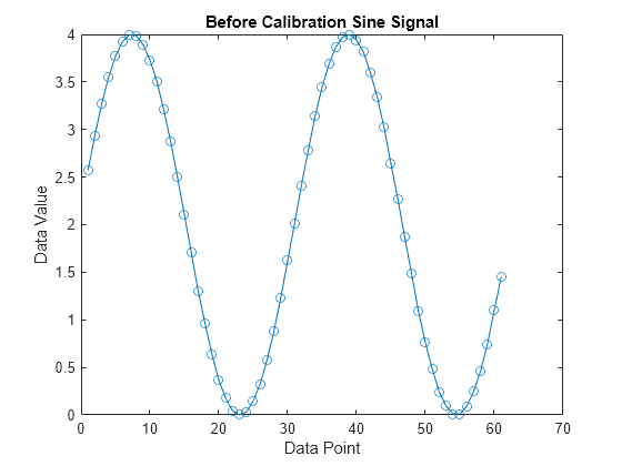
绘制应用了 Gain 值的 Sine 测量变量值。Sine 测量变量值反映了在 Gain 的值设置为 2 的情况下有所增加,如前所示。
plot(sineBeforeCalibration, "o-");
title("Before Calibration Sine Signal");
xlabel("Data Point");
ylabel("Data Value");
标定增益特征变量
使用 writeCharacteristic 将新值写入特征变量 Gain,并使用 readCharacteristic 执行读取以验证更改。Gain 的新值是 5,这意味着新 Gain 值 5 将会增加 Sine 测量变量值。
writeCharacteristic(xcpCh, "Gain", 5);
newGain = readCharacteristic(xcpCh, "Gain")
newGain =
5
获取标定后的测量变量值
从 XCP 服务器采集数据
使用 startMeasurement 函数和 stopMeasurement 函数短时间运行 DAQ 列表。
startMeasurement(xcpCh);
pause(6);
stopMeasurement(xcpCh);
检索 Sine 测量变量数据
要检索 DAQ 列表所采集的 Sine 测量变量数据,请使用 readDAQList 函数,然后从输出 DAQ 列表中检索 Sine 信号。通道中有一个测量变量列表,因此测量变量列表的索引应为 1。
DAQList = readDAQList(xcpCh);
listIndex = 1;
sineAfterCalibration = DAQList{listIndex}.Sine;
绘制 Sine 测量变量值
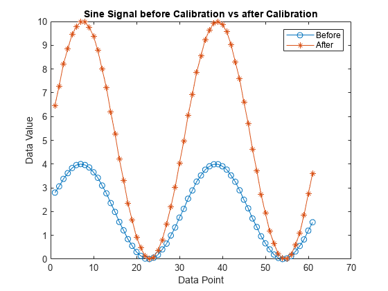
绘制 SineAfterCalibration 测量变量值与 SineBeforeCalibration 测量变量值的关系图。现在,Sine 测量变量信号具有更高的振幅,因为特征变量 Gain 的值在标定后设置为 5。
plot(sineBeforeCalibration, "o-"); hold on;
plot(sineAfterCalibration, "*-"); hold off;
title("Sine Signal before Calibration vs after Calibration");
legend("Before", "After");
xlabel("Data Point");
ylabel("Data Value");
标定特征变量一维查找表
查找表在工业中广泛用于控制参数。因此,下节介绍如何在 XCP Sample 服务器中使用轴 xData 和特征变量 yData 标定一维查找表。
使用 readAxis 和 readCharacteristic 读取当前一维查找表特征变量,然后绘制映射图。下表将输入值有效地映射到了对应的输出值。
inputBreakpoints = readAxis(xcpCh, "xData")inputBreakpoints = 1×8
0 1 2 3 4 5 6 7
outputPoints = readCharacteristic(xcpCh, "yData")outputPoints = 1×8
100 101 102 103 104 105 106 107
plot(inputBreakpoints, outputPoints);
title("Initial 1-D Look-up Table Map");
xlabel("Input Value");
ylabel("Output Value");

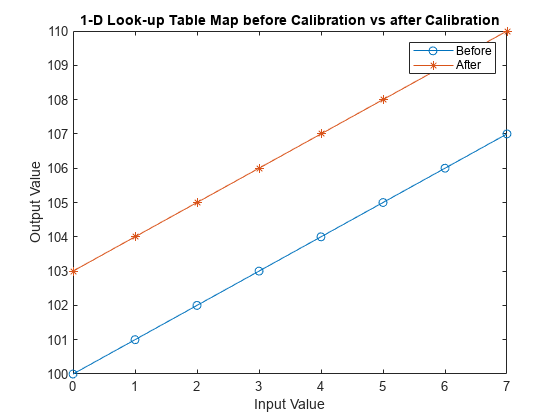
使用 writeCharacteristic 将新数据点写入一维查找表的输出。
writeCharacteristic(xcpCh, "yData", 103:110);使用 readAxis 和 readCharacteristic 读取新一维查找表数据,然后绘制映射。现在,新的 yData 特征变量已设置为更高的值。
xData = readAxis(xcpCh, "xData");
newOutputPoints = readCharacteristic(xcpCh, "yData")
newOutputPoints = 1×8

   103   104   105   106   107   108   109   110
plot(inputBreakpoints, outputPoints, "o-"); hold on
plot(inputBreakpoints, newOutputPoints, "*-"); hold off;
title("1-D Look-up Table Map before Calibration vs after Calibration");
legend("Before", "After");
xlabel("Input Value");
ylabel("Output Value");
断开与服务器的连接
要使与服务器的通信处于非活动状态,请使用 disconnect 函数。断开连接后,XCP 服务器可以安全关闭。
disconnect(xcpCh);
清理
clear sampleServer a2lInfo