Analytic Wavelets Using the Dual-Tree Wavelet Transform

This example shows how to create approximately analytic wavelets using the dual-tree complex wavelet transform. The FIR filters in the two filter banks must be carefully constructed in order to obtain an approximately analytic wavelet transform and derive the benefits of the dual-tree transform.

Create the zero signal 256 samples in length. Obtain two dual-tree transforms of the zero signal down to level 5. By default, dualtree uses the default near-symmetric biorthogonal filter pair nearsym5_7 for level 1, and the orthogonal Q-shift Hilbert wavelet filter pair of length 10 for levels greater than 1.

x = zeros(256,1);
[a1,d1] = dualtree(x,'Level',5);
[a2,d2] = dualtree(x,'Level',5);

Set a single level-five detail coefficient in each of the two trees to 1 and invert the transform to obtain the wavelets.

d1{5}(5) = 1;
d2{5}(5) = 1i;
wav1 = idualtree(a1,d1);
wav2 = idualtree(a2,d2);

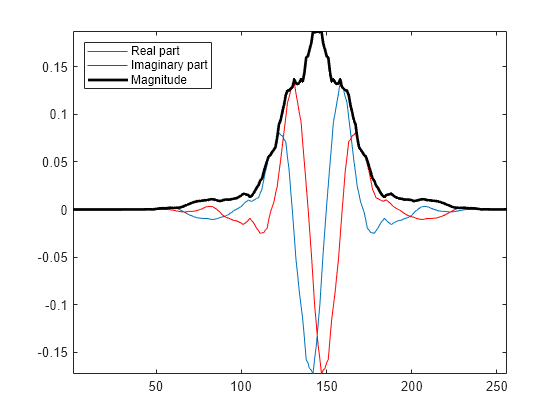
Form the complex wavelet using the first tree as the real part and the second tree as the imaginary part. Plot the real and imaginary parts of the wavelet.

analwav = wav1+1i*wav2;
plot(real(analwav))
hold on
plot(imag(analwav),'r')
plot(abs(analwav),'k','linewidth',2)
axis tight
legend('Real part','Imaginary part','Magnitude','Location','Northwest')

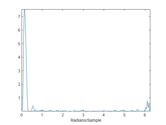
Fourier transform the analytic wavelet and plot the magnitude.

zdft = fft(analwav);
domega = (2*pi)/length(analwav);
omega = 0:domega:(2*pi)-domega;
clf;
plot(omega,abs(zdft))
xlabel('Radians/Sample')
axis tight

The Fourier transform of the wavelet has support on essentially only half of the frequency axis.