Detecting Discontinuities and Breakdown Points
Signals with very rapid evolutions such as transient signals in dynamic systems may undergo abrupt changes such as a jump, or a sharp change in the first or second derivative. Fourier analysis is usually not able to detect those events. The purpose of this example is to show how analysis by wavelets can detect the exact instant when a signal changes and also the type (a rupture of the signal, or an abrupt change in its first or second derivative) and amplitude of the change. In image processing, one of the major applications is edge detection, which also involves detecting abrupt changes.
Frequency Breakdown
Short wavelets are often more effective than long ones in detecting a signal rupture. Therefore, to identify a signal discontinuity, we will use the Haar wavelet. The discontinuous signal consists of a slow sine wave abruptly followed by a medium sine wave.
load freqbrk
x = freqbrk;
Compute the multilevel 1-D wavelet decomposition at level 1.
level = 1;
[c,l] = wavedec(x,level,'haar');
Extract the detail coefficients at level 1 from the wavelet decomposition and visualize the result. Interpolate the detail coefficients so they and the signal have the same length.
d1 = detcoef(c,l,level);
subplot(2,1,1)
plot(x)
subplot(2,1,2)
plot(interpft(d1,2*length(d1)))
ylabel('d1')

The first-level details (d1) show the discontinuity most clearly, because the rupture contains the high-frequency part. The discontinuity is localized very precisely around time = 500.
The presence of noise makes identification of discontinuities more complicated. If the finer levels of the decomposition can be used to eliminate a large part of the noise, the rupture is sometimes visible at coarser levels in the decomposition.
Second Derivation Breakdown
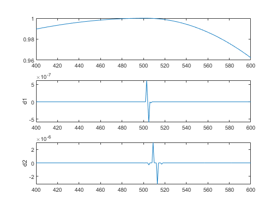
The purpose of this example is to show how analysis by wavelets can detect a discontinuity in one of a signal's derivatives. The signal, while apparently a single smooth curve, is actually composed of two separate exponentials.
load scddvbrk;
x = scddvbrk;
level = 2;
[c,l] = wavedec(x,level,'db4');
[d1,d2] = detcoef(c,l,1:level);
d1up = dyadup(d1,0);
d2up = dyadup(dyadup(d2,0),0);
subplot(3,1,1)
plot(x)
xlim([400 600])
subplot(3,1,2)
plot(d1up)
ylabel('d1')
xlim([400 600])
subplot(3,1,3)
plot(d2up)
ylabel('d2')
xlim([400 600])

We have zoomed in on the middle part of the signal to show more clearly what happens around time = 500. The details are high only in the middle of the signal and are negligible elsewhere. This suggests the presence of high-frequency information — a sudden change or discontinuity — around time = 500.
Note that to detect a singularity, the selected wavelet must be sufficiently regular, which implies a longer filter impulse response. Regularity can be an important criterion in selecting a wavelet. We have chosen to use db4, which is sufficiently regular for this analysis. Had we chosen the Haar wavelet, the discontinuity would not have been detected. If you try repeating this analysis using the Haar wavelet at level two, you will notice that the details are equal to zero at time = 500.
Edge Detection
For images, a two-dimensional discrete wavelet transform leads to a decomposition of approximation coefficients at level j in four components: the approximation at level j+1, and the details in three orientations (horizontal, vertical, and diagonal).
load tartan;
level = 1;
[c,s] = wavedec2(X,level,'coif2');
[chd1,cvd1,cdd1] = detcoef2('all',c,s,level);
subplot(1,2,1)
image(X)
colormap(map)
title('Original Image')
subplot(1,2,2)
image(chd1)
colormap(map)
title('Horizontal Edges')

subplot(1,2,1)
image(cvd1)
colormap(map)
title('Vertical Edges')
subplot(1,2,2)
image(cdd1)
colormap(map)
title('Diagonal Edges')
