Lifting a Filter Bank

Open Live Script

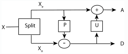
This example shows how to use lifting to progressively change the properties of a perfect reconstruction filter bank. The following figure shows the three canonical steps in lifting: split, predict, and update.

The first step in lifting is simply to split the signal into its even- and odd-indexed samples. These are called polyphase components and that step in the lifting process is often referred to as the "lazy" lifting step because you really are not doing that much work. You can do this in MATLAB® by creating a "lazy" lifting scheme using liftingScheme with default settings.

LS = liftingScheme;

Use the lifting scheme to obtain the level 1 wavelet decomposition of a random signal.

x = randn(8,1);
[ALazy,DLazy] = lwt(x,'LiftingScheme',LS,'Level',1);

MATLAB indexes from 1 so ALazy contains the odd-indexed samples of x and DLazy contains the even-indexed samples. Most explanations of lifting assume that the signal starts with sample 0, so ALazy would be the even-indexed samples and DLazy the odd-indexed samples. This example follows that latter convention. The "lazy" wavelet transform treats one half of the signal as wavelet coefficients, DLazy, and the other half as scaling coefficients, ALazy. This is perfectly consistent within the context of lifting, but a simple split of the data does really sparsify or capture any relevant detail.

The next step in the lifting scheme is to predict the odd samples based on the even samples. The theoretical basis for this is that most natural signals and images exhibit correlation among neighboring samples. Accordingly, you can "predict" the odd-indexed samples using the even-indexed samples. The difference between your prediction and the actual value is the "detail" in the data missed by the predictor. That missing detail comprises the wavelet coefficients.

In equation form, you can write the prediction step as $d_{j} (n) = d_{j - 1} (n) - P (a_{j - 1})$ where $d_{j - 1} (n)$ are the wavelet coefficients at the finer scale and $a_{j - 1}$ is some number of finer-scale scaling coefficients. $P (\cdot)$ is the prediction operator.

Add a simple (Haar) prediction step that subtracts the even (approximation) coefficient from the odd (detail) coefficient. In this case the prediction operator is simply $(- 1) a_{j - 1} (n)$ . In other words, it predicts the odd samples based on the immediately preceding even sample.

ElemLiftStep = liftingStep('Type','predict','Coefficients',-1,'MaxOrder',0);

The above code says "create an elementary prediction lifting step using a polynomial in $z$ with the highest power $z^{0}$ . The coefficient is -1. Update the lazy lifting scheme.

LSN = addlift(LS,ElemLiftStep);

Apply the new lifting scheme to the signal.

[A,D] = lwt(x,'LiftingScheme',LSN,'Level',1);

Note that the elements of A are identical to those in ALazy. This is expected because you did not modify the approximation coefficients.

[A ALazy]

ans = 4×2

    0.5377    0.5377
   -2.2588   -2.2588
    0.3188    0.3188
   -0.4336   -0.4336

If you look at the elements of D{1}, you see that they are equal to DLazy{1}-ALazy.

Dnew = DLazy{1}-ALazy;
[Dnew D{1}]

ans = 4×2

    1.2962    1.2962
    3.1210    3.1210
   -1.6265   -1.6265
    0.7762    0.7762

Compare Dnew to D. Imagine an example where the signal was piecewise constant over every two samples.

v = [1 -1 1 -1 1 -1];
u = repelem(v,2)

u = 1×12

     1     1    -1    -1     1     1    -1    -1     1     1    -1    -1

Apply the new lifting scheme to u.

[Au,Du] = lwt(u,'LiftingScheme',LSN,'Level',1);
Du{1}

You see that all the Du are zero. This signal has been compressed because all the information is now contained in 6 samples instead of 12 samples. You can easily reconstruct the original signal

urecon = ilwt(Au,Du,'LiftingScheme',LSN);
max(abs(u(:)-urecon(:)))

ans = 
0

In your prediction step, you predicted that the adjacent odd sample in your signal had the same value as the immediately preceding even sample. Obviously, this is true only for trivial signals. The wavelet coefficients capture the difference between the prediction and the actual values (at the odd samples). Finally, use the update step to update the even samples based on differences obtained in the prediction step. In this case, update using the following $a_{j} (n) = a_{j - 1} (n) + d_{j - 1} (n) / 2$ . This replaces each even-indexed coefficient by the arithmetic average of the even and odd coefficients.

elsUpdate = liftingStep('Type','update','Coefficients',1/2,'MaxOrder',0);
LSupdated = addlift(LSN,elsUpdate);

Obtain the wavelet transform of the signal with the updated lifting scheme.

[A,D] = lwt(x,'LiftingScheme',LSupdated,'Level',1);

If you compare A to the original signal, x, you see that the signal mean is captured in the approximation coefficients.

[mean(A) mean(x)]

ans = 1×2

   -0.0131   -0.0131

In fact, the elements of A are easily obtainable from x by the following.

n = 1;
for ii = 1:2:numel(x)
    meanz(n) = mean([x(ii) x(ii+1)]);
    n = n+1;
end

Compare meanz and A. As always, you can invert the lifting scheme to obtain a perfect reconstruction of the data.

xrec = ilwt(A,D,'LiftingScheme',LSupdated);
max(abs(x-xrec))

ans = 
2.2204e-16

It is common to add a normalization step at the end so that the energy in the signal ( $ℓ^{2}$ norm) is preserved as the sum of the energies in the scaling and wavelet coefficients. Without this normalization step, the energy is not preserved.

norm(x,2)^2

ans = 
11.6150

norm(A,2)^2+norm(D{1},2)^2

ans = 
16.8091

Add the necessary normalization step.

LSsteps = LSupdated.LiftingSteps;
LSscaled = liftingScheme('LiftingSteps',LSsteps,'NormalizationFactors',[sqrt(2)]);
[A,D] = lwt(x,'LiftingScheme',LSscaled,'Level',1);
norm(A,2)^2+norm(D{1},2)^2

ans = 
11.6150

Now the $ℓ^{2}$ norm of the signal is equal to the sum of the energies in the scaling and wavelet coefficients. The lifting scheme you developed in this example is the Haar lifting scheme.

Wavelet Toolbox™ supports many commonly used lifting schemes through liftingScheme with predefined predict and update steps, and normalization factors. For example, you can obtain the Haar lifting scheme with the following.

lshaar = liftingScheme('Wavelet','haar');

To see that not all lifting schemes consist of single predict and update lifting steps, examine the lifting scheme that corresponds to the bior3.1 wavelet.

lsbior3_1 = liftingScheme('Wavelet','bior3.1')

lsbior3_1 = 
 	 Wavelet               : 'bior3.1' 
	 LiftingSteps          : [3 × 1] liftingStep 
	 NormalizationFactors  : [2.1213 0.4714] 
	 CustomLowpassFilter   : [  ] 


 Details of LiftingSteps :
            Type: 'update'
    Coefficients: -0.3333
        MaxOrder: -1

            Type: 'predict'
    Coefficients: [-0.3750 -1.1250]
        MaxOrder: 1

            Type: 'update'
    Coefficients: 0.4444
        MaxOrder: 0