Load Multivariate Signal

Load the multivariate signal by typing the following at the MATLAB(R) prompt:

 load ex4mwden
 whos

  Name           Size            Bytes  Class     Attributes

  covar          4x4               128  double              
  x           1024x4             32768  double              
  x_orig      1024x4             32768  double              

Usually, only the matrix of data x is available. Here, we also have the true noise covariance matrix covar and the original signals x_orig. These signals are noisy versions of simple combinations of the two original signals. The first signal is "Blocks" which is irregular, and the second one is "HeavySine" which is regular, except around time 750. The other two signals are the sum and the difference of the two original signals, respectively. Multivariate Gaussian white noise exhibiting strong spatial correlation is added to the resulting four signals, which produces the observed data stored in x.

Perform Simple Multiscale PCA

Multiscale PCA combines noncentered PCA on approximations and details in the wavelet domain and a final PCA. At each level, the most significant principal components are selected.

First, set the wavelet parameters:

level = 5;
wname = 'sym4';

Then, automatically select the number of retained principal components using Kaiser's rule, which retains components associated with eigenvalues exceeding the mean of all eigenvalues, by typing:

npc = 'kais';

Finally, perform multiscale PCA:

[x_sim, qual, npc] = wmspca(x ,level, wname, npc);

Display the Original and Simplified Signals

To display the original and simplified signals type:

kp = 0;
for i = 1:4 
    subplot(4,2,kp+1), plot(x (:,i)); axis tight; 
    title(['Original signal ',num2str(i)])
    subplot(4,2,kp+2), plot(x_sim(:,i)); axis tight;
    title(['Simplified signal ',num2str(i)])
    kp = kp + 2;
end

We can see that the results from a compression perspective are good. The percentages reflecting the quality of column reconstructions given by the relative mean square errors are close to 100%.

qual

qual = 1×4

   98.0545   93.2807   97.1172   98.8603

Improve the First Result by Retaining Fewer Principal Components

We can improve the results by suppressing noise, because the details at levels 1 to 3 are composed essentially of noise with small contributions from the signal. Removing the noise leads to a crude, but efficient, denoising effect.

The output argument npc is the number of retained principal components selected by Kaiser's rule:

npc

npc = 1×7

     1     1     1     1     1     2     2

For d from 1 to 5, npc(d) is the number of retained noncentered principal components (PCs) for details at level d. npc(6) is the number of retained non-centered PCs for approximations at level 5, and npc (7) is the number of retained PCs for final PCA after wavelet reconstruction. As expected, the rule keeps two principal components, both for the PCA approximations and the final PCA, but one principal component is kept for details at each level.

To suppress the details at levels 1 to 3, update the npc argument as follows:

npc(1:3) = zeros(1,3);
npc

npc = 1×7

     0     0     0     1     1     2     2

Then, perform multiscale PCA again by typing:

[x_sim, qual, npc] = wmspca(x, level, wname, npc);

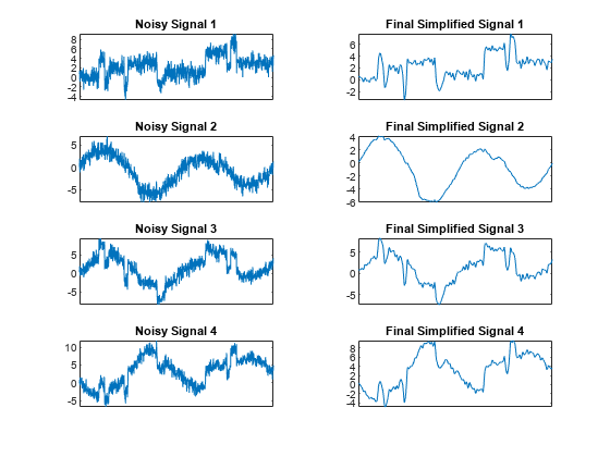
Display the Original and Final Simplified Signals

To display the original and final simplified signals type:

kp = 0;
for i = 1:4 
    subplot(4,2,kp+1), plot(x (:,i)); axis tight;
    title(['Original signal ',num2str(i)])
    subplot(4,2,kp+2), plot(x_sim(:,i)); axis tight; 
    title(['Simplified signal ',num2str(i)])
    kp = kp + 2;
end

As we can see above, the results are improved.

More about Multiscale Principal Components Analysis

More about multiscale PCA, including some theory, simulations and real examples, can be found in the following reference:

Aminghafari, M.; Cheze, N.; Poggi, J-M. (2006), "Multivariate denoising using wavelets and principal component analysis," Computational Statistics & Data Analysis, 50, pp. 2381-2398.