Scale-Localized Volatility and Correlation

There are a number of different variations of the wavelet transform. This example focuses on the maximal overlap discrete wavelet transform (MODWT). The MODWT is an undecimated wavelet transform over dyadic (powers of two) scales, which is frequently used with financial data. One nice feature of the MODWT for time series analysis is that it partitions the data variance by scale. To illustrate this, consider the quarterly chain-weighted U.S. real GDP data for 1974Q1 to 2012Q4. The data were transformed by first taking the natural logarithm and then calculating the year-over-year difference. Obtain the MODWT of the real GDP data down to level six with the 'db2' wavelet. Examine the variance of the data and compare that to the variances by scale obtained with the MODWT.

load GDPcomponents
realgdpwt = modwt(realgdp,'db2',6);
vardata = var(realgdp,1);
varwt = var(realgdpwt,1,2);

In vardata you have the variance for the aggregate GDP time series. In varwt you have the variance by scale for the MODWT. There are seven elements in varwt because you obtained the MODWT down to level six resulting in six wavelet coefficient variances and one scaling coefficient variance. Sum the variances by scale to see that the variance is preserved. Plot the wavelet variances by scale ignoring the scaling coefficient variance.

totalMODWTvar = sum(varwt);
bar(varwt(1:end-1,:))
AX = gca;
AX.XTickLabels = {'[2 4)','[4 8)','[8 16)','[16 32)','[32 64)','[64 128)'};
xlabel('Quarters')
ylabel('Variance')
title('Wavelet Variance by Scale')

Because this data is quarterly, the first scale captures variations between two and four quarters, the second scale between four and eight, the third between 8 and 16, and so on.

From the MODWT and a simple bar plot, you see that cycles in the data between 8 and 32 quarters account for the largest variance in the GDP data. If you consider the wavelet variances at these scales, they account for 57% of the variability in the GDP data. This means that oscillations in the GDP over a period of 2 to 8 years account for most of the variability seen in the time series.

Wavelet analysis can often reveal changes in volatility not evident in aggregate data. Begin with a plot of the GDP data.

helperFinancialDataExample1(realgdp,years,'Year over Year Real U.S. GDP')

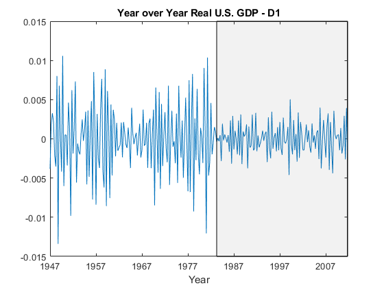
The shaded region is referred to as the "Great Moderation" signifying a period of decreased macroeconomic volatility in the U.S. beginning in the mid 1980s.

Examining the aggregate data, it is not clear that there is in fact reduced volatility in this period. Use wavelets to investigate this by first obtaining a multiresolution analysis of the real GDP data using the 'db2' wavelet down to level 6.

realgdpwt = modwt(realgdp,'db2',6,'reflection');
gdpmra = modwtmra(realgdpwt,'db2','reflection');

Plot the level-one details, D1. These details capture oscillations in the data between two and four quarters in duration.

helperFinancialDataExample1(gdpmra(1,:),years,...
    'Year over Year Real U.S. GDP - D1')

Examining the level-one details, it appears there is a reduction of variance in the period of the Great Moderation.

Test the level-one wavelet coefficients for significant variance changepoints.

[pts_Opt,kopt,t_est] = wvarchg(realgdpwt(1,1:numel(realgdp)),2);
years(pts_Opt)

ans =

        1982

There is a variance changepoint identified in 1982. This example does not correct for the delay introduced by the 'db2' wavelet at level one. However, that delay is only two samples so it does not appreciably affect the results.

To assess changes in the volatility of the GDP data pre and post 1982, split the original data into pre- and post-changepoint series. Obtain the wavelet transforms of the pre and post datasets. In this case, the series are relatively short so use the Haar wavelet to minimize the number of boundary coefficients. Compute unbiased estimates of the wavelet variance by scale and plot the result.

tspre = realgdp(1:pts_Opt);
tspost = realgdp(pts_Opt+1:end);
wtpre = modwt(tspre,'haar',5);
wtpost = modwt(tspost,'haar',5);
prevar = modwtvar(wtpre,'haar','table');
postvar = modwtvar(wtpost,'haar','table');
xlab = {'[2Q,4Q)','[4Q,8Q)','[8Q,16Q)','[16Q,32Q)','[32Q,64Q)'};
helperFinancialDataExampleVariancePlot(prevar,postvar,'table',xlab)
title('Wavelet Variance By Scale');
legend('Pre 1982 Q2','Post 1982 Q2','Location','NorthWest');

From the preceding plot, it appears there are significant differences between the pre-1982Q2 and post-1982Q2 variances at scales between 2 and 16 quarters.

Because the time series are so short in this example, it can be useful to use biased estimates of the variance. Biased estimates do not remove boundary coefficients. Use a 'db2' wavelet filter with four coefficients.

wtpre = modwt(tspre,'db2',5,'reflection');
wtpost = modwt(tspost,'db2',5,'reflection');
prevar = modwtvar(wtpre,'db2',0.95,'EstimatorType','biased','table');
postvar = modwtvar(wtpost,'db2',0.95,'EstimatorType','biased','table');
xlab = {'[2Q,4Q)','[4Q,8Q)','[8Q,16Q)','[16Q,32Q)','[32Q,64Q)'};
figure;
helperFinancialDataExampleVariancePlot(prevar,postvar,'table',xlab)
title('Wavelet Variance By Scale');
legend('Pre 1982 Q2','Post 1982 Q2','Location','NorthWest');

The results confirm our original finding that the Great Moderation is manifested in volatility reductions over scales from 2 to 16 quarters.

You can also use wavelets to analyze correlation between two datasets by scale. Examine the correlation between the aggregate data on government spending and private investment. The data cover the same period as the real GDP data and are transformed in the exact same way.

[rho,pval] = corrcoef(privateinvest,govtexp);

Government spending and personal investment demonstrate a weak, but statistically significant, negative correlation of -0.215. Repeat this analysis using the MODWT.

wtPI = modwt(privateinvest,'db2',5,'reflection');
wtGE = modwt(govtexp,'db2',5,'reflection');
wcorrtable = modwtcorr(wtPI,wtGE,'db2',0.95,'reflection','table');
display(wcorrtable)

wcorrtable =

  6x6 table

          NJ      Lower        Rho         Upper        Pvalue      AdjustedPvalue
          ___    ________    ________    __________    _________    ______________

    D1    257    -0.29187    -0.12602      0.047192       0.1531         0.7502   
    D2    251    -0.54836    -0.35147      -0.11766    0.0040933       0.060171   
    D3    239    -0.62443    -0.35248    -0.0043207     0.047857        0.35175   
    D4    215    -0.70466    -0.32112       0.20764      0.22523        0.82773   
    D5    167    -0.63284     0.12965       0.76448      0.75962              1   
    S5    167    -0.63428     0.12728       0.76347      0.76392              1   

The multiscale correlation available with the MODWT shows a significant negative correlation only at scale 2, which corresponds to cycles in the data between 4 and 8 quarters. Even this correlation is only marginally significant when adjusting for multiple comparisons.

The multiscale correlation analysis reveals that the slight negative correlation in the aggregate data is driven by the behavior of the data over scales of four to eight quarters. When you consider the data over different time periods (scales), there is no significant correlation.

With financial data, there is often a leading or lagging relationship between variables. In those cases, it is useful to examine the cross-correlation sequence to determine if lagging one variable with respect to another maximizes their cross-correlation. To illustrate this, consider the correlation between two components of the GDP -- personal consumption expenditures and gross private domestic investment.

piwt = modwt(privateinvest,'fk8',5);
pcwt = modwt(pc,'fk8',5);
figure;
modwtcorr(piwt,pcwt,'fk8')

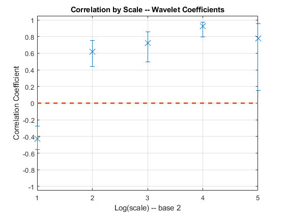
Personal expenditure and personal investment are negatively correlated over a period of 2-4 quarters. At longer scales, there is a strong positive correlation between personal expenditure and personal investment. Examine the wavelet cross-correlation sequence at the scale representing 2-4 quarter cycles.

[xcseq,xcseqci,lags] = modwtxcorr(piwt,pcwt,'fk8');
zerolag = floor(numel(xcseq{1})/2)+1;
plot(lags{1}(zerolag:zerolag+20),xcseq{1}(zerolag:zerolag+20));
hold on;
plot(lags{1}(zerolag:zerolag+20),xcseqci{1}(zerolag:zerolag+20,:),'r--');
xlabel('Lag (Quarters)');
grid on;
title('Wavelet Cross-Correlation Sequence -- [2Q,4Q)');

The finest-scale wavelet cross-correlation sequence shows a peak positive correlation at a lag of one quarter. This indicates that personal investment lags personal expenditures by one quarter.

References:

Aguigar-Conraria, L. Martins. M.F., and Soares, M.J. "The Yield Curve and the Macro-Economy Across Time and Frequencies.", Journal of Economic Dynamics and Control, 36, 12, 1950-1970, 2012.

Crowley, P.M. "A Guide to Wavelets for Economists.", Journal of Economic Surveys, 21, 2, 207-267, 2007.

Gallegati, M and Semmler, W. (Eds.) "Wavelet Applications in Economics and Finance", Springer, 2014.

Percival, D.B. and Walden, A.T. "Wavelet Methods for Time Series Analysis", Cambridge University Press, 2000.