Scaling Function and Wavelet

This example uses wavefun to demonstrate how the number of vanishing moments in a biorthogonal filter pair affects the smoothness of the corresponding dual scaling function and wavelet. While this example uses wavefun for a biorthogonal wavelet, 'bior3.7', you can also use wavefun to obtain orthogonal scaling and wavelet functions.

First, obtain the scaling and wavelet filters and look at the number of vanishing moments in the wavelets. This is equivalent to looking at the number of zeros at -1+i0 in the dual filter.

[LoD,HiD,LoR,HiR] = wfilters('bior3.7');

If you have the Signal Processing Toolbox™, you can use zplane to look at the number of zeros at -1+i0 for both the decomposition and reconstruction filters.

zplane(LoD); title('Decomposition Filter');

figure;
zplane(LoR); title('Reconstruction Filter');

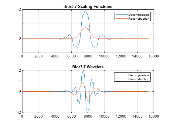
If you zoom in on the region around -1+i0, you find there are 7 zeros in the decomposition filter and 3 zeros in the reconstruction filter. This has important consequences for the smoothness of the corresponding scaling functions and wavelets. For biorthogonal wavelets, the more zeros at -1+i0 in the lowpass filter, the smoother the opposite scaling function and wavelet is. In other words, more zeros in the decomposition filter implies a smoother reconstruction scaling function and wavelet. Conversely, more zeros in the reconstruction filter implies a smoother decomposition scaling function and wavelet.

Use wavefun to confirm this. For orthogonal and biorthogonal wavelets, wavefun works by reversing the Mallat algorithm. Specifically, the algorithm starts with a single wavelet or scaling coefficient at the coarsest resolution level and reconstructs the wavelet or scaling function to the specified finest resolution level. Generally, 8 to 10 levels is sufficient to get an accurate representation of the scaling function and wavelet.

[phiD,psiD,phiR,psiR] = wavefun('bior3.7',10);
subplot(2,1,1)
plot([phiD' phiR']); grid on;
title('Bior3.7 Scaling Functions');
legend('Decomposition','Reconstruction');
subplot(2,1,2)
plot([psiD' psiR']); grid on;
title('Bior3.7 Wavelets');
legend('Decomposition','Reconstruction');

Because there are more than twice the number of zeros at -1+i0 for the lowpass decomposition filter, the dual (reconstruction) scaling function and wavelet are much smoother than the analysis (decomposition) scaling function and wavelet.