Mobility Models in Wireless Network Simulations

In wireless network simulations, mobility models define how nodes, such as mobile devices or vehicles, move over time. Accurate mobility modeling is essential for evaluating network performance in a wide range of wireless systems, including wireless local area network (WLAN), 5G, Bluetooth, mobile ad hoc networks (MANETs), and vehicular networks. Among the various mobility models, three of most frequently used are random walk, random waypoint, and constant velocity.

Random walk — Simulates highly unpredictable, memoryless movement.
Random waypoint — Represents the destination-oriented movement with optional pauses typical of human behavior.
Constant velocity — Captures steady motion, such as that of vehicles traveling on a highway.

With Wireless Network Toolbox™, you can implement these mobility models using the nodeMobilityRandomWalk, nodeMobilityRandomWaypoint, and nodeMobilityConstantVelocity objects, respectively. The toolbox also supports custom mobility models through the wnet.Mobility base class for advanced or scenario-specific behaviors. This topic explains the concepts underlying these mobility model objects.

Random Walk Mobility Model

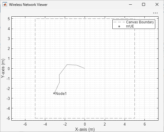
Imagine a mobile node beginning its journey at a starting point. It picks a random direction and speed, then moves forward for a fixed distance or a certain period of time. Upon reaching that distance or time, the node instantly picks another random direction and speed, continuing its motion without interruption. In the random walk mobility model, the node keeps moving, constantly changing its direction and speed at each step. Its path features abrupt turns and unpredictable shifts, making it hard to anticipate where the node might go next. This figure shows an example of how a 5G user equipment node travels according to the random walk model.

A mobile node travels according to the random walk model.

Mathematical Representation of Random Walk Mobility Model

Let the position of the node at time t be $(x (t), y (t))$ . If the node moves with speed v in direction θ for a time interval Δt, its position coordinates after that interval are $(x (t + Δ t), y (t + Δ t))$ , where:

$x (t + Δ t) ＝ x (t) + (v \times Δ t \times c o s (θ))$

and

$y (t + Δ t) ＝ y (t) + (v \times Δ t \times s i n (θ))$

Here:

v follows a uniform distribution: $v \sim U (v_{min}, v_{max}) .$
θ follows a uniform distribution: $θ \sim U (0, 2 π)$

Bounding Mobility Region

In real-world scenarios, nodes typically remain within a bounded area, such as a room, building, or geographic region. To reflect this, simulations often implement the random walk mobility model within a rectangular or circular region. This ensures that node movement remains realistic and constrained, which is important for accurate simulation and analysis.

Bounding Mobility Within Rectangle. Consider a node moving inside a rectangular region defined by $x_{min} \leq x \leq x_{m a x} $ , $y_{min} \leq y \leq y_{max}$ , as shown in this diagram.

If the straight-line motion from $(x (t), y (t))$ to the expected new position goes outside this rectangle, the node must bounce off the boundary. To find where this happens, compute the time at which the line of the moving node intersects each of the sides of the rectangle. The equations for position during the motion step are:

$x (t + t') = x (t) + v_{x} t'$ .

$y (t + t') ＝ y (t) + v_{y} t'$ ,

where $v_{x} ＝ v \times c o s (θ)$ , $v_{y} ＝ v \times s i n (θ)$ , and t′ varies from 0 to Δt.

You can then use these equations to calculate the time at which the node reaches each side of the rectangle.

To calculate when the node reaches the right side ( $x = x_{\max}$ ) of the rectangle:
$t_{r i g h t} ＝ \frac{( x_{m a x} - x (t))}{v_{x}}$ .
The corresponding y-coordinate is $y_{r i g h t} ＝ y (t) + v_{y} t_{r i g h t}$ .
This intersection is valid if $y_{\min} \leq y_{r i g h t} \leq y_{\max}$ .
To calculate when the node reaches the left side ( $y = y_{m a x}$ ) of the rectangle:
$t_{l e f t} ＝ \frac{(x_{m i n} - x (t))}{v_{x}}$ .
The corresponding y-coordinate is $y_{l e f t} ＝ y (t) + v_{y} t_{l e f t}$ .
This intersection is valid if $y_{m i n} \leq y_{l e f t} \leq y_{m a x}$ .
To calculate when the node reaches the top side ( $y = y_{m a x}$ ) of the rectangle:
$t_{t o p} ＝ \frac{(y_{m a x} - y (t))}{v_{y}}$ .
The corresponding x-coordinate is $x_{t o p} ＝ x (t) + v_{x} t_{t o p}$ .
This intersection is valid if $x_{m i n} \leq x_{t o p} \leq x_{m a x}$ .
To calculate when the node reaches the bottom side ( $y = y_{m i n}$ ) of the rectangle:
$t_{b o t t o m} ＝ \frac{(y_{m i n} - y (t))}{v_{y}} $ .
The corresponding x-coordinate is $x_{b o t t o m} ＝ x (t) + v_{x} t_{b o t t o m}$ .
This intersection is valid if $x_{m i n} \leq x_{b o t t o m} \leq x_{m a x}$ .

If several intersections are valid, the node reaches the one that occurs first in time. Let t_hit be the smallest positive time among the valid ones. The exact intersection point is then: $(x_{h i t} , y_{h i t}) = (x (t) + v_{x} t_{h i t} , y (t) + v_{y} t_{h i t })$ . If $t_{hit} < Δ t$ , the node reaches the boundary within the step. The remaining time after the node intersects the boundary is $Δ t_{r e m} ＝ Δ t - t_{h i t }$ . The node continues moving inside the rectangle in the reflected direction for the remaining time.

If the node hits a vertical boundary (the left or right side of the rectangle), its horizontal motion reverses: v_x′ ＝ −v_x and v_y′ ＝ v_y. If the node hits a horizontal boundary (the top or bottom of the rectangle), its vertical motion reverses: v_x′ ＝ v_x, and v_y′ ＝ −v_y.

After reflection, the node moves inside the rectangle again during the remaining time Δt_rem.

Bounding Mobility Within Circle. Consider a wireless node traveling in a 2-D region defined by a circle, as shown in this figure.

Let the circle have a center $C = (c_{x}, c_{y})$ and a radius R. When the point moves, it might reach or go beyond the circular boundary.

Given the position p of the node, let the next position of the node be p_next and the velocity before reflection v be (v_x, v_y). The intended next position without considering the boundary is:

$p_{n e x t} = p + v Δ t$ .

The distance from the next point to the center is $d = ‖ p_{n e x t} - C ‖$ . If $d \leq R$ , the point is still inside the circle. If $d > R$ , the point has crossed the boundary.

To place the point exactly on the circular boundary, project it radially inward:

$p_{p r o j} ＝ C + R \frac{(p_{n e x t} - C)}{ ∥ p_{n e x t } - C ∥}$ .

For a circle, the normal vector always points radially outward. At the boundary point p_proj, the outward unit normal is

$n = \frac{(p_{n e x t} - C)}{ ∥ p_{n e x t } - C ∥} = (\frac{1}{R}) (p_{n e x t} - C)$ .

You can then compute the reflected velocity as:

$v' = v - 2 (v \cdot n) n$

In this equation, $(v \cdot n)$ extracts the normal component of the velocity.

Random Waypoint Mobility Model

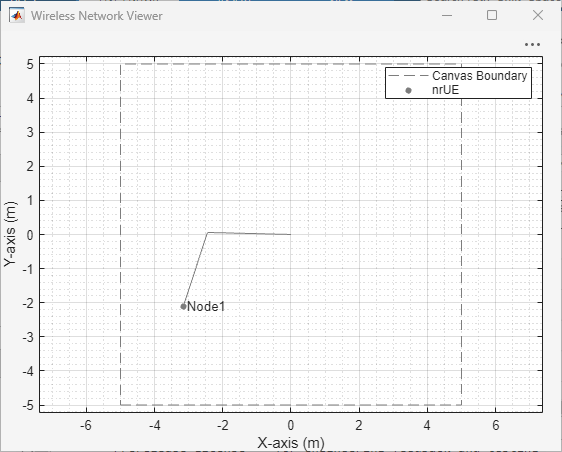
In the random waypoint model, mobile nodes simulate movement by alternating between travel and pause periods. A node begins by remaining stationary for a brief duration, known as the pause time. After the pause, the node randomly selects a new destination and moves toward it at a randomly chosen speed, which lies between a predefined minimum and maximum. Once it reaches the destination, the node pauses again before repeating the process, selecting a new target location and speed and continuing its journey. This cycle continues throughout the simulation. This figure shows an example of how a 5G user equipment node moves according to the random waypoint model.

Random waypoint

Mathematical Representation of Random Waypoint Mobility Model

Consider at any simulation time t, the position of the node is $p (t) = [x (t), y (t), z (t)]$ and its velocity is vector $v (t) = [v_{x} (t), v_{y} (t), v_{z} (t)]$ . Consider motion that is only in the horizontal plane. The vertical coordinate z remains constant throughout the simulation. The node also has a current waypoint, $p_{w p}$ , which defines the destination for the ongoing movement phase.

The simulation region can be rectangular or circular. For a rectangular region defined by a center $(x_{c}, y_{c})$ , width W, and height H, the lower-left lies at

$(x_{c} - \frac{W}{2}, y_{c} - \frac{W}{2})$ .

The simulation selects a waypoint uniformly within this region by generating two independent random variables $U_{1}$ and $U_{2}$ , each uniformly distributed over [ 0, 1] and computing

$x = x_{c} - \frac{W}{2} + W U_{1}$ , $y = y_{c} - \frac{H}{2} + H U_{2}$ .

For a circular region defined by the center $(x_{c}, y_{c})$ and radius R, the simulation selects the waypoint using polar coordinates. It generates two independent uniform random variables $U_{1}$ and $U_{2}$ and computes

$r = R U_{1}$ , $θ = 2 π U_{2}$ ,

which yield the waypoint coordinates

$x = x_{c} + r \cos (θ)$ , $y = y_{c} + r \sin (θ)$ .

After selecting a waypoint, the simulation computes the straight-line distance between the current position $p_{0}$ and the waypoint $p_{w p}$ using the Euclidean norm,

$D = ‖ p_{w p} - p_{0} ‖$ .

This distance determines both the direction of motion and the time required to reach the waypoint.

The simulation selects the node speed from a predefined range, $[v_{\min}, v_{\max}]$ . When the limits differ, it draws the speed uniformly from this interval according to

$v = v_{\min} + (v_{\max} - v_{\min}) U$ ,

where the random variable U is uniformly distributed over [0, 1]. When the limits are equal, the node moves at a constant speed equal to that value. The simulation then computes the velocity vector to align with the direction toward the waypoint,

$v = \frac{v}{D} (p_{w p} - p_{0})$ ,

ensuring straight-line motion at constant speed.

The time required to reach the waypoint is

$T_{r e a c h} = \frac{D}{v}$ .

During the movement phase, the node follows uniform linear motion. For any time increment $Δ t$ , the node updates its position as

$p (t + Δ t) = p (t) + v Δ t$ ,

and accumulates the traveled distance as

$d (t + Δ t) = d (t) + v Δ t$ .

The node does not accelerate. The velocity remains constant during movement.

Upon reaching the waypoint, the node enters a pause phase of fixed duration. During this interval, the node remains at the waypoint,

$p (t) = p_{w p}$ ,

and its velocity becomes zero,

$v (t) = 0$ .

After the pause ends, the simulation selects a new waypoint and the node resumes movement.

Constant Velocity Mobility Model

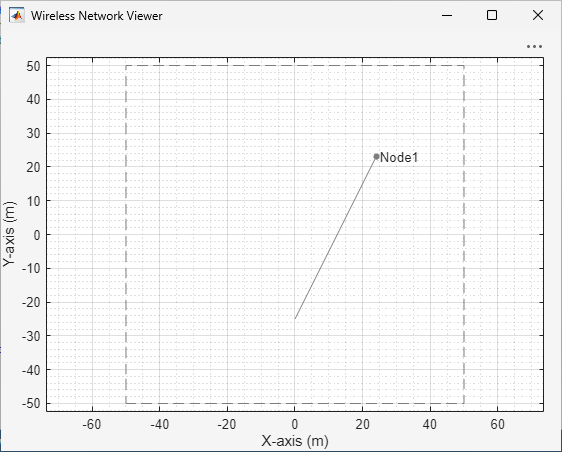
The constant velocity mobility model describes a scenario where mobile nodes move continuously in a fixed direction at a constant speed. Once a node begins moving, it maintains its velocity, both speed and direction, without pausing or changing direction, as shown in this figure.

Constant Velocity Mobility Model

Custom Mobility Model

A custom mobility model is a user-defined way to simulate the movement of wireless nodes, such as vehicles or mobile devices. For instance, if you want to study how vehicular mobility impacts the performance of vehicle-to-vehicle (V2V) communication, you can develop a tailored vehicular mobility model. You can use the wnet.Mobility base class from Wireless Network Toolbox to define your custom mobility model. For more information about how to create a custom mobility model and add it to a wireless node, see Create and Add Custom Mobility Model to Wireless Nodes.

Mobility Models in Wireless Network Simulations

Random Walk Mobility Model

Mathematical Representation of Random Walk Mobility Model

Bounding Mobility Region

Random Waypoint Mobility Model

Mathematical Representation of Random Waypoint Mobility Model

Constant Velocity Mobility Model

Custom Mobility Model

See Also

Objects

Classes