Building Deployable Applications for Evaluating PK/PD Drug Efficacy
By Anita Gajjala and Asawari Samant, MathWorks
Pharmacokinetic/pharmacodynamic (PK/PD) and systems pharmacology models are important tools for evaluating drugs in development. Using MATLAB® and SimBiology®, researchers can build and characterize such models either in a graphical environment or using programmatic tools. They can use preclinical data to mathematically describe the dynamic in vivo behavior of new drug candidates, and make predictions and extrapolations in humans based on model simulations. They can then share these models to enable fellow clinicians, biologists, and researchers to better evaluate the efficacy and safety metrics of various dosing strategies and explore what-if scenarios in different patient subpopulations.
In certain cases, it may not be practical to share SimBiology models directly. For example, your colleagues may lack access to, or be unfamiliar with, MATLAB and SimBiology, or you may wish to lock down the model and its characterization so that other users cannot inadvertently change it.
MATLAB Compiler™ lets you deploy a SimBiology model as part of a standalone MATLAB application. You can build a custom graphical interface that other researchers can use to set up and run model simulations. You can then compile the application to enable researchers to use it without installing MATLAB or SimBiology.
Using an oncology model developed by Koch, Walz, Lahu, and Schropp1 as an example, this article describes a workflow for developing and deploying an application for simulating a mechanistic PK/PD model built using SimBiology2.
The sample model and the deployable app are available for download.
Oncology Model Overview
The example in this article is based on the Koch et al. oncology model, which is used to characterize tumor growth over time in response to either monotherapy treatment with a single drug, or combination therapy involving simultaneous administration of two drugs.
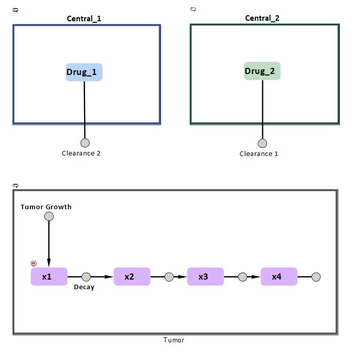
The SimBiology implementation of the Koch et al. oncology model is shown in Figure 13. The plasma concentration of both drugs is described by independent one-compartment PK models with linear elimination routes. The tumor growth model is represented in the Tumor compartment. The rate of the Decay reaction depends on the plasma concentration of Drug A and Drug B and an interaction parameter. When the plasma concentration of the drugs falls to zero, the tumor dynamics is described by the Tumor Growth process. The tumor weight is defined as the sum of the growing and decaying tumor states, i.e. x1+ x2+ x3+ x4.
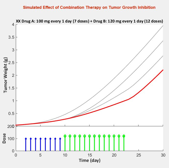
Model simulations make it possible to analyze the effect of various combination dosing strategies on tumor suppression (Figure 2).
Preparing the Model for Deployment
In order to share the SimBiology model using MATLAB Compiler we first create an exported model4.
We load the SimBiology model into MATLAB using sbioloadproject.
>> sbioloadproject('TumorGrowthModel.sbproj'); % Load the Model
We use export and save to create the exported SimBiology model and save it as a MAT file, which will be loaded into the deployed application.
>> exportedModel = export(m1); % Create the Exported Model

>> save modelFile.mat exportedModel % Save the exported model
Note that exported SimBiology models have a limited set of accessible properties. In addition, some model features, including reactions, rules, and events, cannot be changed in the exported version.
Building an Interface to the Model
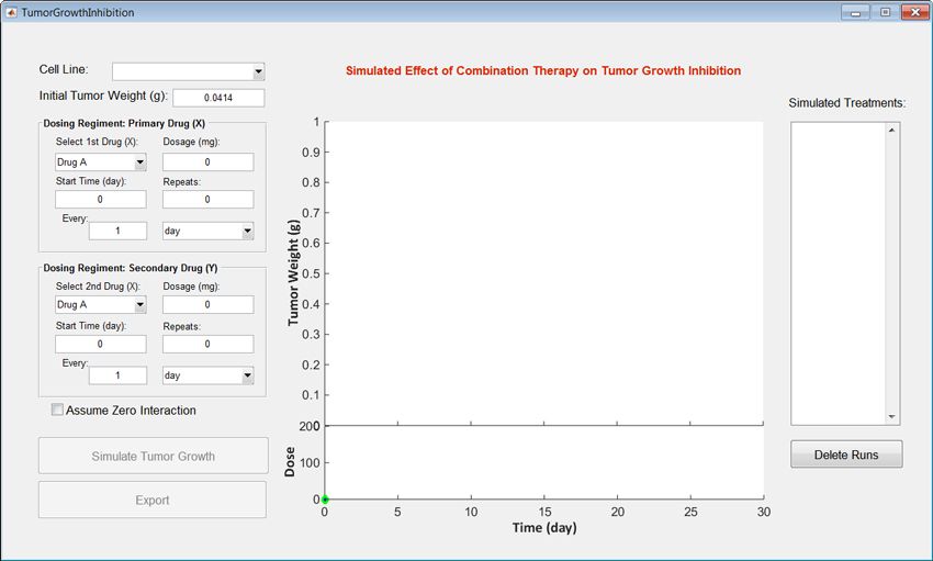
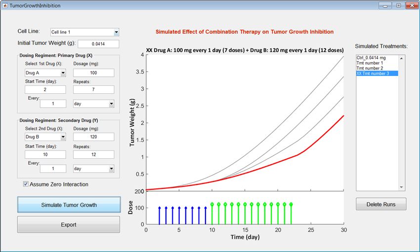
After creating an exported SimBiology model, we build a custom MATLAB interface. The interface will enable non-modelers and researchers without access to MATLAB to adjust model parameters, apply dosing schedules, and run simulations (Figure 3).
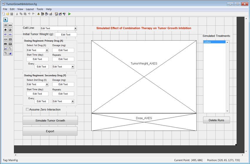
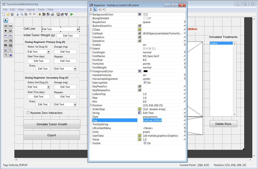
Using MATLAB graphical user interface design environment (GUIDE) tools, we lay out the interface by dragging components from the palette into the layout area (Figure 4).
We need to modify individual properties of each component. For example, we need to update the Tag property for interface elements so that these elements can be easily accessed programmatically. Using a naming convention, such as <Name>_<Type>, improves code readability (Figure 5).
Programming Functions to Access the Exported SimBiology Model
In a MATLAB desktop-based workflow, applications are coded to access a non-exported SimBiology model. In preparation for deployment, we need to update the code to use the exported SimBiology model.
The first step is to indicate to MATLAB Compiler that the application uses an exported SimBiology model. We do this by adding a directive (via the %#function pragma) in the GUIDE-generated MATLAB file, TumorGrowthInhibition.m, which is linked to the GUIDE FIG-file that we saved.
function varargout = TumorGrowthInhibition(varargin)

%#function SimBiology.export.Model
When the end user interacts with an interface control object, such as a menu or a button, in your application, specific functions, or callbacks, are invoked. Next, we will modify the callback functions to use the exported model.
In the sample app we will modify five callbacks to prepare the model for deployment:
TumorGrowthInhibition_OpeningFcn, CellLine_POPUP_Callback, InitialTumorWeight_EDIT_Callback, Dosage1_EDIT_Callback, and SimTumorGrowth_PUSHBUTTON_Callback.
TumorGrowthInhibition_OpeningFcn is the opening function in the example application. It loads the model and initializes doses, model parameters, and other properties in the code. The initial (non-deployed) version uses sbioloadproject to load the model into MATLAB and sbiodose or getdose to create or edit existing dose objects.
function
TumorGrowthInhibition_OpeningFcn(hObject,eventdata,handles,varargin)

% <SNIP>

% Create and initialize dose -- non-deployed version

    % Load project
    proj = sbioloadproject('TumorGrowthModel.sbproj');
    m1 = proj.m1;

    % Get dose 1
    d1 = getdose(m1,'Drug A');
    % Get dose 2
    d2 = getdose(m1,'Drug B');

% <SNIP>
For deployed applications, we load the exported model from a MAT file (instead of using sbioloadproject). We use getdose to update the existing dose objects attached to the exported model since new dose objects cannot be added to exported models.
function
TumorGrowthInhibition_OpeningFcn(hObject,eventdata,handles,varargin)

% <SNIP>

% Create and initialize dose –- deployed version
    % Load model
    proj = load('modelFile.mat');
    m1 = proj.exportedModel;

    % Get dose 1
    d1 = getdose(m1,'Drug A');
    % Get dose 2
    d2 = getdose(m1,'Drug B');


% <SNIP>
CellLine_POPUP_Callback is invoked when the user selects a cell line from the pop-up menu. This function is responsible for setting the cell line parameters appropriately based on the user’s selection. In the non-exported version of the model, this is done by selecting the appropriate variant with a single call to sbioselect.
function CellLine_POPUP_Callback(hObject,eventdata,handles)

% <SNIP>

% Set the appropriate cell line name invariant –- non-deployed version

  	    cellLine = sbioselect(model,'type','variant','name',cellLineName);

% <SNIP>
SimBiology model variants cannot be used with exported models. So for exported models, we use ValueInfo and getIndex to get and set individual model parameters that make up a model variant.
function CellLine_POPUP_Callback(hObject,eventdata,handles)

% <SNIP>

% Set the appropriate cell line parameters –- deployed version

    % Get current L1 and L0 values
    L1 = model.ValueInfo(getIndex(model, 'L1'));
    L0 = model.ValueInfo(getIndex(model, 'L0'));

    switch cellLineName
        case 'Cell line 1'
            L0.InitialValue = 0.141;
            L1.InitialValue = 0.282;
        case 'Cell line 2'
            L0.InitialValue = 0.142;
            L1.InitialValue = 0.284;
        case 'Cell line 3'
            L0.InitialValue = 0.143;
            L1.InitialValue = 0.286;
        otherwise
            %
    end

% <SNIP>
InitialTumorWeight_EDIT_Callback is invoked when the user specifies an initial tumor weight (w0). Like CellLine_POPUP_Callback, the non-deployed version of this callback uses sbioselect to set the parameter value in the model.
function InitialTumorWeight_EDIT_Callback(hObject,eventdata,handles)

% <SNIP>

% Set value of w0 in the model –- non-deployed version

            w0 = sbioselect(model,'type','parameter','name','w0');
            w0.Value = str2double(get(hObject,'String'));

% <SNIP>
As with CellLine_POPUP_Callback, we use ValueInfo and getIndex to set the values in the exported SimBiology models for the deployed application.
function InitialTumorWeight_EDIT_Callback(hObject,eventdata,handles)

% <SNIP>

% Set value of w0 in the model –- deployed version

           w0 = model.ValueInfo(getIndex(model,'w0'));
           w0.InitialValue = str2double(get(hObject,'String'));

% <SNIP>
Dosage1_EDIT_Callback is invoked when the user specifies dosage time units. This callback updates the dose object. Initially this is done by setting the TimeUnits and Interval properties directly.
function Dosage1_EDIT_Callback(hObject,eventdata,handles)

% <SNIP>

% Set dose object’s settings –- non-deployed version
% Set TimeUnits and Interval directly
    dose1.TimeUnits = timeUnits;
    dose1.Interval = str2double(get(handles.EveryValue1_EDIT,'String'));
    % Convert StartTime from day to new TimeUnits
    dose1.StartTime =
sbiounitcalculator('day',dose1.TimeUnits,str2double(get(handles.StartTime1_
EDIT,'String')));

% <SNIP>
In deployed applications, TimeUnits is a read-only property of dose objects, so it cannot be set directly. We use sbiounitcalculator &to convert the dose interval to the dose’s existing time units.
function Dosage1_EDIT_Callback(hObject,eventdata,handles)

% <SNIP>

% Set dose object’s settings –- deployed version
% Cannot set TimeUnits; use sbiounitcalculator to convert Interval
    dose1.Interval =
sbiounitcalculator('day',dose1.TimeUnits,str2double(get(handles.EveryValue1_
EDIT,'String')));
    % Convert StartTime from day to new TimeUnits
    dose1.StartTime =
sbiounitcalculator('day',dose1.TimeUnits,str2double(get(handles.StartTime1_
EDIT,'String')));

% <SNIP>
SimTumorGrowth_PUSHBUTTON_Callback is invoked when the user clicks the Simulate Tumor Growth button. This callback runs the simulation with the appropriate parameter values and dosing schedules to calculate the tumor weight evolution over time. In the non-deployed version of the model, it calls sbiosimulate.
function SimTumorGrowth_PUSHBUTTON_Callback(hObject,eventdata,handles)

% <SNIP>

% Simulate model & get tumor profile –- non-deployed version

    sd = sbiosimulate(model,'',[cellLine,phiVar],[dose1,dose2]);
    [currResults.Time,currResults.Tumor] = selectbyname(sd,'w');

% <SNIP>
For exported models, we replace sbiosimulate with simulate.
function SimTumorGrowth_PUSHBUTTON_Callback(hObject,eventdata,handles)

% <SNIP>

% Simulate model & get tumor profile –- deployed version

    sd = simulate(model,initValues,[dose1,dose2]);
    [currResults.Time,currResults.Tumor] = selectbyname(sd,'w');

% <SNIP>
Setting Up Report Generation
Using MATLAB Report Generator™ we generate a document that captures the model’s PK/PD response, model parameters, and dosing schedule. Our application will generate a PDF document called “myreport.pdf”. This callback uses the new Document Object Model (DOM) API available in MATLAB Report Generator 4.0 (R2014b), which lets us to build reports programmatically.
% --- Executes on button press in Export_PUSHBUTTON.
function Export_PUSHBUTTON_Callback(hObject, eventdata, handles)
% hObject    handle to Export_PUSHBUTTON (see GCBO)
% eventdata  reserved - to be defined in a future version of MATLAB
% handles    structure with handles and user data (see GUIDATA)

% <SNIP>

% Generate report
    %%%%%% Initialize %%%%%%
    % Import DOM settings
    import mlreportgen.dom.*;

    % Make it deployable for use with MATLAB Compiler
    makeDOMCompilable();

    % Create document
    rpt = Document('myReport', 'pdf');

    %%%%%% Create main section %%%%%%
    % <SNIP>
    h = Heading(2, 'Simulated Effect of Combination Therapy on Tumor Growth');
    b = Border();
    b.BottomStyle = 'single';
    b.BottomColor = 'LightGray';
    b.BottomWidth = '1pt';
    h.Style = [h.Style {Color('DarkOrange'), b}];
    append(rpt, h);

    p = append(rpt, Paragraph('*Automatically generated using MATLAB Report
Generator 4.0 (R2014b).'));
    p.Style = {FontFamily('Arial'), FontSize('10pt')};

    %%%%%% Create settings section %%%%%%
    % <SNIP>
    tableData = {...
        'Cell Line:', cellLineName{1};
        'Initial Tumor Weight (g):', initialTumorWeight};
    table = Table(size(tableData,1));
    append(rpt, table);

    %%%%%% Create results section %%%%%%
    % <SNIP>
    hFig = figure;

    % Tumor Weight Axes
    hAxes = copyobj(handles.TumorWeight_AXES, hFig);
    set(hAxes,'Units','normalized');
    set(hAxes,'Position',[0.15 0.30 0.7 0.6]);

    % Dose Axes
    hAxes = copyobj(handles.Dose_AXES, hFig);
    set(hAxes,'Units','normalized');
    set(hAxes,'Position',[0.15 0.15 0.7 0.15]);

    % Set dimensions in inches
    set(hFig,'Units','inches');
    Pos = get(hFig,'Position');
    set(hFig,'Position',[Pos(1:2) 6 5]);
    set(hFig,'PaperPosition',[0 0 6 5]);

    % Print and append to report
    print(hFig, '-dmeta', 'plot1.emf');
    img = Image('plot1.emf');
    img.Width = '6in';
    img.Height = '5in';
    append(rpt, Paragraph(img));

    %% View report
    close(rpt);
    rptview('myReport', 'pdf');

% <SNIP>
Testing the Application in MATLAB
We execute the TumorGrowthInhibition command to launch the application in MATLAB. When the application launches, we specify the cell line, initial tumor weight, and dosing schedules, then click the Simulate Tumor Growth button to begin the simulation.
The plot displays simulation results for four different treatments (Figure 6).
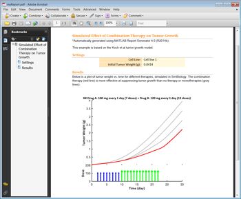
We click the Export button on the interface to generate a PDF file showing the results (Figure 7).
We are now ready to create a standalone application that we can distribute to researchers who do not have MATLAB installed.
Deploying the Application
The following MATLAB commands locate all file and path dependencies and invoke the MATLAB Compiler command to compile the TumorGrowthInhibition.m application for deployment:
% Note, this assumes that all additional applicable files are on path
additionalFiles = [{'modelFile.mat', 'Summary.rpt'} ...
    exportedModel.DependentFiles];

% For the purposes of this example, we programmatically construct the |mcc|
% command:
mccCommand = ['mcc -m TumorGrowthInhibition.m' ...
    sprintf(' -a %s', additionalFiles{:})];

% Execute the |mcc| command.
eval(mccCommand)
Once the compilation is complete, an executable (.exe) is generated for distribution with the MATLAB Compiler Runtime (MCR). The MCR is a set of shared libraries that enables users to execute compiled MATLAB applications on computers that do not have MATLAB installed.
Summary: Applying the Workflow
You can use the process outlined in this article to deploy one of your own SimBiology models as a standalone application. Start by loading the model in MATLAB and creating an exported SimBiology model with the export and save commands. Next, build a simple interface with GUIDE, and program callback functions to access your SimBiology model via interface control elements. Finally, after testing your application in MATLAB, compile it with MATLAB Compiler and retest the resulting executable on a computer that does not have MATLAB installed.
1 Koch, G., Walz A., Lahu, G., and Schropp, J. (2009) Modeling of tumor growth and anticancer effects of combination therapy. Journal of Pharmacokinetics and Pharmacodynamics. 36:179-197.
2 This step was completed by Koch et al, and while this article provides an overview of the approach, the video “Building a Model – Differential Equations | SimBiology Tutorials for QSP, PBPK, and PK/PD Modeling and Analysis” (see below), provides more detail about this step.
3 The underlying rate equations are not shown in Figure 1. Please refer to Koch et. al or the downloadable SimBiology app for model and implementation details.
4 SimBiology project files (*.sbproj) are not compatible with MATLAB Compiler.
Published 2014 - 92233v00
