Improve the Fidelity of Your Simulink Models Using Test Data and Parameter Estimation
By Craig Borghesani, MathWorks and Bora Eryilmaz, MathWorks
For most engineers and scientists, working with a model of a physical system instead of an actual prototype provides a convenient way to experiment with various design and control ideas. The benefits of working with models are well understood in engineering, physical sciences, and economics and are gaining recognition in medicine, biomedical sciences, and finance. However, in order to make full use of models in these areas, the model must accurately represent the behavior of the actual system under study.
Simulink Parameter Estimation is a tool designed to help you calibrate the response of your Simulink model to match the outputs of the physical system or prototype that you are modeling. Thus, it eliminates the need to adjust the model parameters by trial and error or develop your own optimization routines in-house. Using experimental data and state-of-the-art optimization methods, Simulink Parameter Estimation computes your model parameters and initial conditions.
This article describes how to use Simulink Parameter Estimation to estimate the parameters of a multidomain DC servo motor model. We develop the model using the first-principles modeling approach and physical domain modeling tools including Simscape Electrical and SimDriveline. Simulink Parameter Estimation handles the parameter estimation problem, using experimental data collected on the actual system to identify all unknown model parameters.
Modeling and Parameter Estimation
First-principles modeling is a tool-based approach to determining the dynamics of an actual system using basic physical laws to model each component in the system. This enables an engineer to build a model in the same way they would build the actual system: through physical connections rather than equation composition. The first-principles approach enables more engineers to better understand the model without conducting lengthy mathematical calculations—it simplifies the modeling task and saves time and resources.
Simulink is well-suited to first-principles modeling with its graphical environment that represents components such as gains, integrators, and multipliers in a block format. Using physical domain modeling tools enables us to avoid a manual equation-composition process by building models using bodies, joints, gears, clutches, power sources, and resistors.
First-principles models provide important insight into system behavior, but may lack accuracy. It is very important that our model response matches the real-world data. Fortunately, a model developed using a first-principles approach renders the parameters relating to physical quantities readily exposed and available for estimation. We can use parameter estimation to obtain an accurate model of a real system, and an accurate model provides a strong platform for further design or control strategy development.
Example: DC Servo Motor System
A DC servo motor, with its electrical and mechanical components, provides a great example to illustrate multidomain modeling using first principles.
The DC servo motor is part of a larger system that contains the control electronics (H-Bridge) and a disk attached to the motor shaft. Figure 1 shows the overall model, where the Input Signal (V) is the voltage signal applied to the H-bridge circuit, and the Output Signal (deg) is the angular position of the motor shaft.
We develop a first-principles model of the DC motor within the DC servo motor subsystem. We use Simscape Electrical to model the electrical components and SimDriveline to model the mechanical components of the motor. Figure 2 shows the content of the servo motor subsystem.
The DC motor model shows a relationship from current to torque (the green line on the left). The torque causes the shaft of the motor to spin and we have a relationship between this spinning to the Back EMF (electromotive force). The rest of the parameters include a shaft inertia, viscous friction (damping), armature resistance, and armature inductance.
While manufacturers may provide values for some of these quantities, they are only estimates. We want to estimate these parameters as precisely as possible for our model to ascertain whether it is an accurate representation of the actual DC servo motor system. Table 1 lists the model parameters and their initial values.
| Viscous Friction (B) | 0.008 Nms/rad |
| Shaft Inertia (J) | 5.7e-7 kg m^2 |
| Motor Constant (Km) | 0.0134 Vs/rad |
| Armature Inductance (La) | 6.5e-5 H |
| Armature Resistance (Ra) | 1.9 ohm |
When we apply a series of voltage pulses to the motor input, the motor shaft turns in response. However, if the model parameters do not match those of the physical system, the model response will not match that of the actual system, either. Figure 3 shows the current response of our model using the initial parameter values listed in Table 1. It is obvious that we need to estimate our parameters. This is where Simulink Parameter Estimation plays a pivotal role.

Figure 3. Model response using initial motor parameter values.
Using Simulink Parameter Estimation to Improve Your Models
An accurate model requires that its structure resembles that of the actual system. The DC motor model, for example, has a system consisting of an electrical subsystem supplying torque to the motor shaft, and a mechanical subsystem where applied torque results in rotational motion.
We also need to calculate the motor parameter values that we are going to use in the model. Although some model parameters are known, most cases require measurements on the actual system. It may not always be possible to get accurate parameter values by measurement because they can be difficult or time-consuming to measure. For example, in our DC motor model, measuring the torque constant requires a sophisticated measurement setup that may not be readily available.
We can use Simulink Parameter Estimation to estimate our model parameter values. Using input-output data from a physical system or prototype, Simulink Parameter Estimation calculates the unknown parameters and reconciles differences between the model and the actual system. We can input a known range of parameter values and associate test data with input and output signals at any level within the structure of the model.
Note: For details on using Simulink Parameter Estimation, see the product documentation.
Estimating Parameters of the DC Motor Model
A parameter estimation process consists of a number of well-defined steps:
- Collect test data from your system (experiment).
- Specify the parameters to estimate (including initial guesses, parameter bounds, etc.).
- Configure your estimation and run a suitable estimation algorithm.
- Validate the results against other test data sets and repeat above steps if necessary.
Simulink Parameter Estimation provides a graphical user interface (GUI) to help you follow these steps, neatly organize your estimation project, and save it for future work. You can launch this product from the Tools menu of your Simulink model. The tool automatically creates a default estimation project for you (Figure 4).
Importing Experimental Data
The first step in our estimation project is to import the experimental data that we have collected from the actual DC motor system. We import multiple data sets corresponding to various experimental conditions.
Simulink Parameter Estimation provides preprocessing tools such as noise filtering, detrending, splitting, and so forth to prepare data sets for estimation and/or validation. You can import experimental data sets from various sources including MATLAB variables, MAT files, Excel files, or comma-separated-value files. Once you import the data, you can also plot them to confirm that you have the right data sets in your estimation project.
Selecting Parameters for Estimation
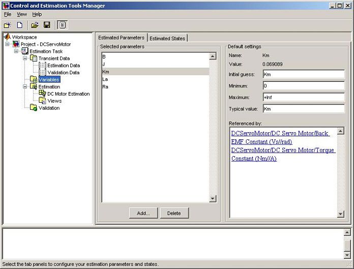
Next, we select the model parameters whose value we want to estimate. The tool automatically recognizes all the parameters that we use in the model and lets us select a subset of them for estimation. Once we select the estimation parameters, we can set initial guesses for the parameter values, as well as the minimum and maximum bounds on these values, as shown in Figure 5.
Simulink Parameter Estimation lets you estimate some or all of these parameters in a manner that best suits your application. For our DC motor example, we will estimate all five parameters of the motor model: B, J, Km, La, and Ra.
Defining an Estimation
Once you import your data and select the parameters to estimate, the next step is to create an estimation node in the GUI tree and configure various options. Each estimation uses your experimental data sets to estimate the parameter that you have selected. However, you have the option of using only some of the data sets for estimation while keeping the others for validation. You can also elect to estimate only a subset of the selected parameters.
Simulink Parameter Estimation also provides various state-of-the-art estimation algorithms. The most common selections include the nonlinear least-squares and Nelder-Mead optimization methods. More information on these algorithms is available in the Optimization Toolbox documentation. You can also use the algorithms in the Genetic Algorithm and Direct Search Toolbox for parameter estimation.
Running the Estimation
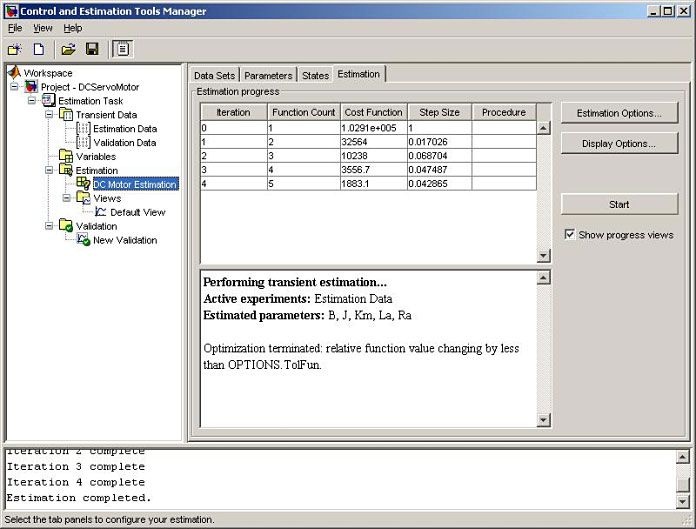
Once we finish configuring our estimation, we can run it and see how Simulink Parameter Estimation adjusts our model parameter values in order to match the model's response with our experimental data sets. Figure 6 shows the GUI while the estimation is running.
While the estimation is running, we can also monitor its progress by creating views (plots) that update at each iteration of the estimation process. Simulink Parameter Estimation creates two views by default. The first view plots the simulation response against the experimental data used for the estimation, as shown in Figure 7. As the parameter values improve, the simulation curve gets closer to the experimental data curve. The second view plots the parameter values at each iteration, as shown in Figure 8. These curves will reach steady-state as the parameter values get closer to their physical values.

Figure 7. Measured vs. simulated response of the DC motor.

Figure 8. Motor parameter trajectories.
Comparing the response of the system before (Figure 3) and after (Figure 7) the estimation process clearly shows that the estimation successfully identified the model parameters and the simulated response accurately matches the experimental data.
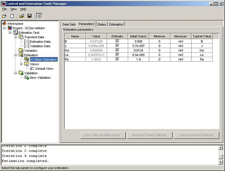
Once the estimation is complete, we can inspect the estimated parameter values (Figure 9). The Value column displays the new parameter values at the end of the estimation.
These parameter values also update in the MATLAB Workspace so that we can use them directly in the Simulink model. Table 2 lists the estimated parameter values.
| Viscous Friction (B) | 0.0373 Nms/rad |
| Shaft Inertia (J) | 8.0e-6 kg m^2 |
| Motor Constant (Km) | 0.0691 Vs/rad |
| Armature Inductance (La) | 9.16e-4 H |
| Armature Resistance (Ra) | 1.95 ohm |
Validation
After completing the estimation, it is important to validate the results against other data sets. A successful estimation should match not only the experimental data that we used for estimation, but also the other data sets that we collected in our experiments.
We used our second data set for validating the estimation results. As Figure 10 shows, the match between the model response and the data set is very good. In fact, the two curves are almost identical for this example.

Figure 10. Validation with the second experimental data set.
Summary
Engineers and scientists across disciplines and industry are well acquainted with the benefits of modeling dynamic systems. They may use either first-principles mathematics or test-data based methods. First-principles models provide important insight into system behavior, but may lack accuracy. Data-driven models provide accurate results, but tend to offer limited understanding of the physics of the system. This article demonstrated the use of Simulink Parameter Estimation to improve the accuracy of a DC Servo Motor model by estimating the model parameters using experimental data.
For another example of first-principles modeling, see Graphical Techniques for Aircraft Dynamic Model Development by Paul A. Barnard.
Published 2005


