Introduction to Motion Planning Algorithms | Motion Planning Hands-on Using RRT Algorithm, Part 1
From the series: Motion Planning Hands-on Using RRT Algorithm
Motion planning lets robots or vehicles plan an obstacle-free path from a start to goal state. Learn some popular motion planning algorithms, how they work, and their applicability in different scenarios.
Discover how the following algorithms work for global and local path planning in reference to suitable applications such as self-driving cars and warehouse robots - Hybrid A*, Probabilistic Roadmaps (PRM), rapidly-exploring random tree (RRT), RRT*, and Trajectory Optimal Frenet.
Learn about various functions with MATLAB® and Navigation Toolbox™ to customize a robot's state space and implement different motion models based on the application.
Published: 10 May 2021
Hello everyone. Welcome to the Hands-on Session on Motion Planning with MATLAB. I am Mihir Acharya, product manager for Autonomous Navigation at Networks. And with me, we have YJ Lim, product manager for Robotics and Autonomous Systems at MathWorks. For any type of autonomous robot, motion planning adds the essential piece in the economy. It helps to find a sequence of valid configuration that moves the robot from a source location to destination. In this session, we will learn about path and motion planning algorithms and how you can use MATLAB and navigation toolbox to quickly implement these algorithms and find a shortest obstacle free path for your robot.
We will see two application examples, where I will cover the example on path planning for mobile robots and VJ will be covering how to do the same for a robot manipulator. In a typical autonomous robot workflow, the perception module provides information on how the environment around the robot looks like. That includes the obstacles that the robot should avoid bumping into. We get the location of the robot at each movement or state from the localization algorithms. Motion planning comes into picture when the robot needs to autonomously navigate from the initial location to the goal location.
Motion planning algorithms, help to plan the shortest obstacle free path to the goal. With MATLAB and Simulink, you can use algorithms such as RRT or hybrid A* for global path planning. And you can use trajectory generation for local re-planning in case there is an unknown obstacle on the way.
Furthermore, we can classify motion planning into three categories including the high level decision making earlier called behavior planning. However, we can also classify the types of motion planning algorithms into search based and sampling based. In this session, we will briefly look at these algorithms and how you can implement the RRT algorithm using the planning infrastructure in MATLAB and navigation toolbox. But let's first go over some of these planning algorithms available in MATLAB.
Once we get a map of the environment, there are two types of methods to solve the path planning problem. One method is to discridize the map into grid cells. And the other method is to randomly sample graph nodes in the map. There are several grid-based algorithms such as A* being one of the most popular ones. I think everyone who is into motion planning have an understanding about the A* algorithm. There is a traditional implementation of A* available in MATLAB with customizable cost and heuristics.
A* works well for only drive or holonomic robots. But what if we want a car like motion? We have a variant of A* that allows us to do that, which is hybrid A*. Hybrid A* is similar to the traditional A* algorithm in how the search space that is xy theta is discridized. But unlike traditional A*, hybrid A*, associates a continuous 3D state of the vehicle or as we call them motion primitives with each grid cell. These motion primitives are checked for collisions in the map using state validators and generates smooth obstacle-free path.
Unlike the traditional A*, hybrid A* is suitable for vehicles with non-holonomic constraints and car-like robots, such as a self-driving car. It also guarantees kinematic feasibility and takes differential constraints into account. That means you can take the orientation and velocity of the vehicle into account. You can give the orientation of the vehicle as an input along with this chart and go locations. And we can see how we get different drivable parts based on different goal orientations. With MATLAB and Simulink, you can
implement hybrid A* with multiple parameters to tune such as length of motion primitives, minimum turn radius, forward backward motion and more.
Grid based algorithms are not suitable for various applications that has high degree of freedoms or when the map size is very large. Storing the grid information for a large map becomes computationally expensive. And this is where the sampling-based planning algorithms are helpful. One of the commonly used sampling-based algorithms is PRM or Probabilistic Roadmap which is a network graph of different possible parts in a map. In the implementation with MATLAB, we first import the binary occupancy map that we created using slam. Then we can inflate that map according to the robot's size to avoid collisions with the walls. Then we randomly sample nodes in the free space and the PRM impact plan object in MATLAB connects them to create a roadmap.
Once the roadmap has been constructed, we can query for a part from a given start location to a given goal location on the map. We can query about multiple times in the same roadmap for different start and goal locations. You can customize the number of nodes and the connection distance to fit the complexity of the map. The PRM implementation in MATLAB is suitable for various types of holonomic mobile robot applications where you want to change to start and go locations without the need of learning the whole map again. For example, a static warehouse environment with no unknown obstacles is a good example.
But in many other cases, the robot is non-holonomic. That is, it has differential constraints and could also involve high dimensional state space with unknown obstacles. Which brings us to RRT or Rapidly-exploring Random Tree algorithm. RRT creates a tree in the stage space with randomly sampled states or nodes. The RRT algorithm is designed for efficiently searching non convex high dimensional spaces. RRT are constructed incrementally in a way that it quickly reduces the expected distance of a randomly chosen node in the tree.
Let's briefly see how the sampling based algorithm works. We first define the state space. With an initial tree T that has start point as one of the nodes in it. To represent the map in a way that the planning algorithm or the planner can understand it, we represent it in the form of a state space. A state of a robot is its position and orientation. And the state space is a set of many possible robot states. An example of state space representation is SE2 state space where the robot can move in a 2-D map with each state holding three variables xy and theta.
Now we randomly sample a state X random in the state space X and we find a node nearest to X random that already exists in the tree. Now this X random can be anywhere in the state space. So we need another node X new between X random and X near to expand the tree. And we repeat this process until we reach the X goal. Every time we sample a new mode node like X new, we also check for collision between the nodes x random and x new. With MATLAB, you can use motion primitives or motion models like leads chip or Dubin scar to generate local motion from one node to another.
RRTs are particularly suitable for path planning problems that involve obstacles and differential constraints. And also for robots with high degrees of freedom such as robot manipulators but they're also equally suitable for mobile robot path planning as well. The RRT algorithm gives a valid path but not necessarily the shortest path, which brings us to RRT*. RRT* is a variant of RRT or I can say it's an optimized version of RRT. RRT* is similar to RRT in how it expands to tree. But it rewires the tree in a way that a given such radius and always tries to find a shorter path from the randomly sampled node back to the start in the tree. This makes RRT* to give an optimal solution and makes it even more feasible for high dimensional problems.
While RRT* finds the shortest path with lesser number of nodes, it is not suitable for non-holonomic vehicles as opposed to RRT. RRT is capable of handling differential constraints. So it depends on your applications to figure out which algorithm will be more suitable. In further session, VJ will also cover bidirectional RRT and explains how that works for robot manipulator. Now let's look at the planning infrastructure available in MATLAB and navigation toolbox for sampling based algorithms such as RRT. We first load an occupancy map of the environment where the robot can check for collisions.
The occupancy map specifies the probability of each cell in the map to be occupied with an obstacle or be a cell with free space. Then we represent the state space using one of the building state space representations such as SE2, SE3 or state space for Dubin's vehicles. Dubin state space is an SE2 form of state space that supports Dubin's motion models. This state space allows the robot to move in Dubin's cars that makes it suitable for car-like motion with ackermans steering. The motion models are available as part segments such as Dubin's connection. After we have done the random sampling of states in the state space, the next step is for the planner to need a state validator.
To understand the validity of a state or the motion between the two states, the planner needs a state validator. For example, a robot state is considered to be valid if the robot is not colliding with any of the obstacle at that given state and also during the motion. The collision of any obstacle and the robot state will make it to be an invalid state. And the planner will avoid to add such a state in the part. Navigation toolbox provides a built in state validators for 2-D and 3-D occupancy maps as well as cost maps.
And finally we define the planner and it finds the path. All the built in state spaces are customizable as per your application. We will see in the example that how we customize them. But you can also build your own custom path planning interfaces with MATLAB and navigation tool box. Using this planning infrastructure, it becomes a matter of few lines of code to implement the RRT algorithm in MATLAB. Here we see the syntax of the planner RRT which takes the state space SE2 or any other state space and state validator for occupancy map as inputs. And then it returns the path states and the solution information as the output. Now I will switch to MATLAB and we will look at the shipping example that shows how to plan paths for mobile robots using the RRT algorithm.


