NR Cell Performance Evaluation with Beam Management
This example models a 5G New Radio (NR) cell with transmit-end beam refinement procedure in the downlink (DL) direction and evaluates the network performance. This example shows how to transmit multiple single-port channel state information reference signal (CSI-RS) resources in different directions for Layer 1 (physical layer) reference signal received power (L1-RSRP) measurements. The 5G base station node (gNB) scheduler uses the L1-RSRP reports to beamform the physical downlink shared channel (PDSCH) transmissions for better signal-to-noise-ratio (SNR) at the user equipment (UE) nodes. You can modify the gNB scheduler to select the beam direction for PDSCH transmissions.
Introduction
Downlink beamforming improves the network performance by utilizing the multi-antenna configuration to focus energy of the signals in a direction which results in better SNR at a UE node. Additionally, beamforming also limits the interference in other directions. For efficient DL beamforming, the gNB relies on the channel state information resource indicator (CRI) and L1-RSRP feedback from the UE nodes. The UE nodes measure the L1-RSRP on multiple CSI-RS resources, where each resource corresponds to one direction, and reports the gNB with the CRI having the highest L1-RSRP.
The example models multiple sets of CSI-RS beams for L1-RSRP measurements. Each set corresponds to a wider synchronization signal block (SSB) beam and contains finer CSI-RS beams within the SSB beam. The example does not model the SSB beam sweeping process for initial acquisition, and assumes the SSB beam associated with each UE node to be the beam with angular range covering the line-of-sight (LOS) path from the gNB.
This example models:
DL channel quality measurement and reporting by UE nodes based on the multi-port CSI-RS received from the gNB. The report includes rank indicator (RI), precoding matrix indicator (PMI), and channel quality indicator (CQI). The example supports Type-1 single-panel codebook for PMI.
DL L1-RSRP measurement and CRI reporting by UE nodes based on the single-port CSI-RS received from the gNB.
Transmit end beam refinement in DL direction using CRI-RSRP feedback.
Single-codeword DL spatial multiplexing to perform multi-layer transmission. Single-codeword limits the number of transmission layers to 4.
Precoding to map the transmission layers to antenna ports.
Digital beamforming of PDSCH based on the CRI feedback from the UE nodes.
Free space path loss (FSPL), additive white Gaussian noise (AWGN), and clustered delay line (CDL) propagation channel model.
Nodes send the control packets (buffer status report (BSR), DL assignment, UL grants, PDSCH feedback, CSI report, and CRI-RSRP reports) out of band, without the need of resources for transmission and assured error-free reception.
MIMO
The key aspects of multiple-input multiple-output (MIMO) include precoding, beamforming, channel measurement and reporting.
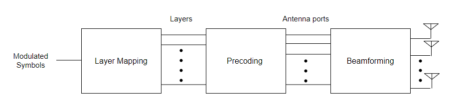
Layer mapping
The layer mapping process maps the modulated symbols of the codeword onto different layers.
Precoding
Precoding, which follows the layer mapping, maps the transmission layers to antenna ports. Precoding applies a precoding matrix to the transmission layers and outputs data streams to the antenna ports.
Beamforming
Beamforming involves the use of multiple radiating elements transmitting the same signal to produce a longer and narrower beam in a particular direction. The higher the number of antennas, the narrower the beamwidth.
Beam management is a set of physical (PHY) layer and medium access control (MAC) layer procedures to acquire and maintain a set of beam pair links (a beam used at the gNB paired with a beam used at a UE node). Three procedures are available for beam management. For more information about these procedures, refer to NR Downlink Transmit-End Beam Refinement Using CSI-RS example.
The current example focuses on the Procedure 2 (P-2) beam measurement and beam reporting procedures. This procedure involves sending single port CSI-RS resources over highly directional beams to each UE node. The UE nodes report the L1-RSRP measurements over each of these resources back to the gNB node. The gNB node uses these measurements to perform transmit beam refinement for all subsequent downlink transmissions intended for the UE node till the next L1-RSRP measurement.
DL Channel Measurement and Reporting
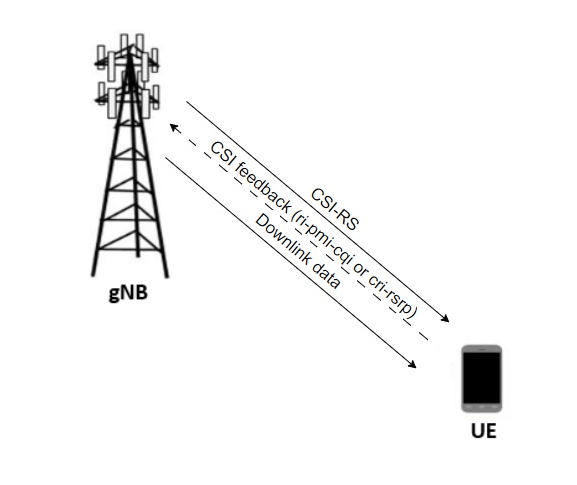
CSI reporting is the process by which a UE node, for DL transmissions, advises a suitable number of transmission layers (rank), PMI, and CQI values to the gNB. The UE node estimates these values by performing channel measurements on its configured CSI-RS resources. For more information about this, see the 5G NR Downlink CSI Reporting example. The gNB scheduler uses this advice to decide the number of transmission layers, precoding matrix, and modulation and coding scheme (MCS) for PDSCHs.
The UE node also uses the CSI report to indicate the CRI, and the L1-RSRP to aid the gNB in transmit beam refinement.
NR Protocol Stack
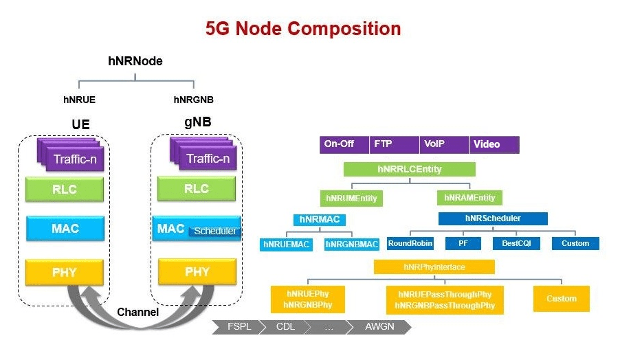
A node (gNB or UE) is a composition of NR stack layers. The helpers hNRGNB and hNRUE create gNB and UE nodes, respectively, containing the radio link control (RLC), MAC and PHY layer. For more information about this, see the NR Cell Performance Evaluation with Physical Layer Integration example.
Scenario Configuration
Configure simulation parameters in the simParameters structure.
rng('default');                  % Reset the random number generator
simParameters = [];              % Clear the simParameters variable
simParameters.NumFramesSim = 10; % Simulation time in terms of number of 10 ms frames
Enable or disable DL beamforming.
enableBeamforming = true;
Specify the azimuth sweep angles and direction of SSBs. The azimuth angle is the angle measured in the horizontal plane, ranging from [-180, 180] and the elevation angle is the angle measured in the vertical plane, ranging from [-90, 90] between the horizontal plane and the LOS point in the Spherical coordinate system.
if enableBeamforming
    % Number of SSBs
    numSSBs = 4;
    % Total azimuthal range for all SSBs corresponding to a 120 degrees sectorized cell
    azSweepRange = [-60, 60];
    validateattributes(azSweepRange,{'numeric'},{'nonempty','real', 'vector', ...
        '>=',-60,'<=',60,'finite'}, ...
        'azSweepRange','azimuthal range');
    % Sweep range for non-overlapping SSB directions
    ssbSweepRange = diff(azSweepRange)/numSSBs;
    % Azimuthal angles for SSB beam sweeping in the azimuthal range
    ssbTxAngles = [-60 -20 20 60];
    % Elevation range for all SSBs sweeping in the azimuthal angles
    elSweepRange = [-45, 0];
end
Specify the number of UE nodes in the cell, assuming that the UE nodes have sequential radio network temporary identifiers (RNTIs) from 1 to simParameters.NumUEs. If you change the number of UE nodes, ensure that the number of rows in simParameters.UEPosition is equal to the value of simParameters.NumUEs.
simParameters.NumUEs = 3;
% Position of the gNB node in (x,y,z) coordinates
simParameters.GNBPosition = [0, 0, 0];
% Specify the UE node position in spherical coordinates (r,azimuth,elevation)
% relative to the gNB. Here 'r' is the distance, 'azimuth' is the angle in the
% horizontal plane and 'elevation' is the angle in the vertical plane. When
% enabling beamforming, ensure that all UE node positions lie within the azimuth
% and elevation range limits of SSBs, as defined in the previous section. It is a matrix of
% size N-by-3, where N represents the number of UE nodes. Row 'i' of the matrix contains
% the coordinates of a UE node with an RNTI 'i'
ueRelPosition = [500, -5, -5;
    500, -60, -30;
    500, -10, -20];
if enableBeamforming
    validateattributes(ueRelPosition(:,2),{'numeric'},{'nonempty','real','vector', ...
        '>=',azSweepRange(1),'<=',azSweepRange(2),'finite'}, ...
        'ueRelPosition(:,2)','azimuth angles');
    validateattributes(ueRelPosition(:,3),{'numeric'},{'nonempty','real','vector', ...
        '>=',elSweepRange(1),'<=',elSweepRange(2),'finite'}, ...
        'ueRelPosition(:,3)','elevation angles');
end
% Convert Spherical to Cartesian coordinates (considering gNB position as origin)
[xPos, yPos, zPos] = sph2cart(deg2rad(ueRelPosition(:, 2)),deg2rad(ueRelPosition(:, 3)), ...
    ueRelPosition(:, 1));
% Global coordinates of the UE nodes
simParameters.UEPosition = [xPos, yPos, zPos] + simParameters.GNBPosition;
% Validate the UE node positions
validateattributes(simParameters.UEPosition, {'numeric'},{'nonempty','real', ...
    'nrows',simParameters.NumUEs,'ncols',3,'finite'}, ...
    'simParameters.UEPosition','UEPosition');
Set the channel bandwidth to 5 MHz and the subcarrier spacing (SCS) to 15 kHz, as defined in 3GPP TS 38.104 Section 5.3.2.
simParameters.NumRBs = 25;
simParameters.SCS = 15;                % kHz
simParameters.DLBandwidth = 5e6;       % Hz
simParameters.ULBandwidth = 5e6;       % Hz
simParameters.DLCarrierFreq = 2.646e9; % Hz
simParameters.ULCarrierFreq = 2.535e9; % Hz
Specify the transmit (Tx) and receive (Rx) antenna panel geometry at the gNB and UE nodes in the format (M,N,P), where M and N are the number of rows and columns in the antenna array, respectively. P is the number of polarizations (1 or 2).
gNBTxArraySize = [2 4 2];
ueRxArraySize = repmat([1 1 2],simParameters.NumUEs,1);
Configure the gNB transmit antenna panel.
lambda = physconst('LightSpeed')/simParameters.DLCarrierFreq;
simParameters.TxAntPanel = phased.NRRectangularPanelArray('ElementSet', ...
    repmat({phased.NRAntennaElement},1,gNBTxArraySize(3)), ...
    'Size',[gNBTxArraySize(1:2) 1 1],'Spacing', ...
    [0.5*lambda 0.5*lambda 1 1]);
Specify the CSI-RS configuration for RI, PMI and CQI measurements.
csirs = cell(1,simParameters.NumUEs);
csirsOffset = [5 6 10 11];
for csirsIdx = 1:simParameters.NumUEs
    csirs{csirsIdx} = nrCSIRSConfig('NID',1,'NumRB',simParameters.NumRBs, ...
        'RowNumber',11,'SubcarrierLocations',[1 3 5 7], ...
        'SymbolLocations',0,'CSIRSPeriod',[20 csirsOffset(csirsIdx)]);
end
simParameters.CSIRSConfig = csirs;
Specify the CSI-RS resource set configuration associated with each SSB for DL beam refinement. Each resource set contains multiple single-port CSI-RS resources, with each resource corresponding to a particular beam direction within the SSB angular range.
if enableBeamforming
    simParameters.NumCSIRSBeams = 4;
    csirsConfigRSRP = cell(1,numSSBs);
    for ssbIdx = 1:numSSBs
        csirsConfig = nrCSIRSConfig;
        csirsConfig.NID = 1;
        csirsConfig.CSIRSType = repmat({'nzp'},1,simParameters.NumCSIRSBeams);
        csirsConfig.CSIRSPeriod = [40 0];
        csirsConfig.Density = repmat({'one'},1,simParameters.NumCSIRSBeams);
        csirsConfig.RowNumber = repmat(2,1,simParameters.NumCSIRSBeams);
        csirsConfig.SymbolLocations = {1,5,6,7};
        csirsConfig.SubcarrierLocations = repmat({ssbIdx-1},1, ...
            simParameters.NumCSIRSBeams);
        csirsConfig.NumRB = simParameters.NumRBs;
        csirsConfigRSRP{ssbIdx} = csirsConfig;
    end
    simParameters.CSIRSConfigRSRP = csirsConfigRSRP;
end
Specify the signal-to-interference-plus-noise ratio (SINR) to a CQI index mapping table for a block error rate (BLER) of 0.1. The lookup table corresponds to the CQI table as per 3GPP TS 38.214 Table 5.2.2.1-3.
simParameters.DownlinkSINR90pc = [-0.4600 4.5400 9.5400 14.0500 16.540 19.0400 ...
    20.5400 23.0400 25.0400 27.4300 29.9300 30.4300 ...
    32.4300 35.4300 38.4300];
Specify the gNB transmit power.
simParameters.GNBTxPower = 34; % In dBmConfigure the channel model.
channelModelDL = cell(1,simParameters.NumUEs);
waveformInfo = nrOFDMInfo(simParameters.NumRBs,simParameters.SCS);
dlchannel = nrCDLChannel('DelayProfile','CDL-D','DelaySpread',300e-9);
for ueIdx = 1:simParameters.NumUEs
    cdl = hMakeCustomCDL(dlchannel);
    % Configure the channel seed based on the UE number
    % Independent fading for each UE
    cdl.Seed = cdl.Seed + (ueIdx - 1);
    % Compute the LOS angle from gNB to UE
    [~,depAngle] = rangeangle(simParameters.UEPosition(ueIdx, :)', ...
        simParameters.GNBPosition');
    % Configure the azimuth and zenith angle offsets for this UE
    cdl.AnglesAoD(:) = cdl.AnglesAoD(:) + depAngle(1);
    % Convert elevation angle to zenith angle
    cdl.AnglesZoD(:) = cdl.AnglesZoD(:) - cdl.AnglesZoD(1) + (90 - depAngle(2));
    % Compute the range angle from UE to gNB
    [~,arrAngle] = rangeangle(simParameters.GNBPosition',...
        simParameters.UEPosition(ueIdx, :)');
    % Configure the azimuth and zenith arrival angle offsets for this UE
    cdl.AnglesAoA(:) = cdl.AnglesAoA(:) - cdl.AnglesAoA(1) + arrAngle(1);
    % Convert elevation angle to zenith angle
    cdl.AnglesZoA(:) = cdl.AnglesZoA(:) - cdl.AnglesZoA(1) + (90 - arrAngle(2));
    cdl.CarrierFrequency = simParameters.DLCarrierFreq;
    cdl.TransmitAntennaArray = simParameters.TxAntPanel;
    cdl.ReceiveAntennaArray.Size = [ueRxArraySize(ueIdx, :) 1 1];
    cdl.SampleRate = waveformInfo.SampleRate;
    channelModelDL{ueIdx} = cdl;
end
Initialize the beamforming weights table for DL beam refinement. It contains the steering vectors corresponding to direction of various CSI-RS beams across all the SSBs. It is of size M x N, where M represents number of transmit antenna elements and N represents number of CSI-RS beams of all SSBs. The gNB PHY stores this table. For each PDSCH, the scheduler selects a column index in this table (corresponding to the beam direction) and conveys the same to the PHY layer.
% Number of transmit antennas
numTxAntennas = prod(gNBTxArraySize);
if enableBeamforming
    enableVerticalBeamSweep = true;
    simParameters.BeamWeightTable = zeros(numTxAntennas, ...
        simParameters.NumCSIRSBeams*numSSBs);
    txArrayStv = phased.SteeringVector('SensorArray',simParameters.TxAntPanel, ...
        'PropagationSpeed',physconst('LightSpeed'), ...
        'IncludeElementResponse',true);
    azBW = beamwidth(simParameters.TxAntPanel,simParameters.DLCarrierFreq, ...
        'Cut','Azimuth');
    elBW = beamwidth(simParameters.TxAntPanel,simParameters.DLCarrierFreq, ...
        'Cut','Elevation');
    for beamIdx = 1:numSSBs
        % Obtain the azimuthal sweep range for every SSB based on the SSB transmit
        % beam direction and its beamwidth in the azimuth plane
        azSweepRangeSSB = ssbTxAngles(beamIdx) + [-ssbSweepRange/2 ssbSweepRange/2];
        % Obtain the azimuth and elevation angle pairs for all CSI-RS transmit beams
        csirsBeamAng = hGetBeamSweepAngles(simParameters.NumCSIRSBeams,azSweepRangeSSB, ...
            elSweepRange,azBW,elBW,enableVerticalBeamSweep);
        for csirsBeamIdx = 1:simParameters.NumCSIRSBeams
            simParameters.BeamWeightTable(:, simParameters.NumCSIRSBeams*(beamIdx-1) ...
                + csirsBeamIdx) = txArrayStv(simParameters.DLCarrierFreq, ...
                csirsBeamAng(:,csirsBeamIdx))/sqrt(numTxAntennas);
        end
    end

    % Initialize the beam indices for all the UE nodes with highest L1-RSRP (for visualization purpose)
    beamIndices = -1*ones(1,simParameters.NumUEs);
end
Specify the scheduling strategy and the maximum limit on the RBs allotted for PDSCH. The transmission limit applies only to new transmissions and not to the retransmissions.
% Supported scheduling strategies: 'PF', 'RR', and 'BestCQI'
simParameters.SchedulerStrategy = 'PF';
simParameters.RBAllocationLimitDL = 15; % For PDSCH
Logging and visualization configuration
The CQIVisualization and RBVisualization parameters control the display of the CQI visualization and the RB assignment visualization respectively. To enable the RB visualization plot, set the RBVisualization field to true.
simParameters.CQIVisualization = true;
simParameters.RBVisualization = false;
Set the enableTraces to true to log the traces. Setting enableTraces to false automatically disables CQIVisualization and RBVisualization and does not log the traces in the simulation. However, this can speed up the simulation.
enableTraces = true;
The example updates the metrics plots periodically. Specify the number of updates during the simulation.
simParameters.NumMetricsSteps = 10;
Write the logs to MAT-files. You can use these log files for post-simulation analysis and visualization.
parametersLogFile = 'simParameters';         % For logging the simulation parameters
simulationLogFile = 'simulationLogs';        % For logging the simulation traces
simulationMetricsFile = 'simulationMetrics'; % For logging the simulation metrics
Application traffic configuration
Set the periodic DL application traffic pattern for UE nodes.
% DL application data rate in kilo bits per second (kbps)
dlAppDataRate = 40e3*ones(1,simParameters.NumUEs);
% Validate the DL application data rate
validateattributes(dlAppDataRate,{'numeric'},{'nonempty','vector','numel', ...
    simParameters.NumUEs,'finite','>',0},'dlAppDataRate', ...
    'dlAppDataRate');
Derived Parameters
Compute the derived parameters based on the primary configuration parameters specified in the previous section and set some example-specific constants.
simParameters.DuplexMode = 0;                    % FDD (Value as 0) or TDD (Value as 1)
simParameters.SchedulingType = 0;                % Slot-based scheduling
simParameters.NCellID = 1;                       % Physical cell ID
simParameters.GNBTxAnts = numTxAntennas;
simParameters.UERxAnts = prod(ueRxArraySize,2);
Specify the CSI report configuration.
% [N1 N2] as per 3GPP TS 38.214 Table 5.2.2.2.1-2
csiReportConfig.PanelDimensions = [8 1];
csiReportConfig.CQIMode = 'Wideband';              % 'Wideband' or 'Subband'
% Set codebook mode as 1 or 2. It is applicable only when the number of
% transmission layers is 1 or 2 and the number of CSI-RS ports is greater than 2
csiReportConfig.CodebookMode = 1;
simParameters.CSIReportConfig = {csiReportConfig};
Compute the SSB beam corresponding to each UE node.
if enableBeamforming
    simParameters.SSBIndex = computeSSBToUE(simParameters,ssbTxAngles,ssbSweepRange,ueRelPosition);
end
Compute the number of slots in the simulation.
numSlotsSim = (simParameters.NumFramesSim * 10 * simParameters.SCS)/15;
Set the interval at which the example updates metrics visualization in terms of number of slots. Because this example uses a time granularity of one slot, the MetricsStepSize field must be an integer.
simParameters.MetricsStepSize = ceil(numSlotsSim/simParameters.NumMetricsSteps);
Specify one logical channel for each UE node, and set the logical channel configuration for all nodes (gNB and UE nodes) in the example.
numLogicalChannels = 1;
simParameters.LCHConfig.LCID = 4;
Specify the RLC entity type in the range [0, 3]. The values 0, 1, 2, and 3 indicate the RLC UM unidirectional DL entity, the RLC UM unidirectional UL entity, the RLC UM bidirectional entity, and theRLC AM entity, respectively.
simParameters.RLCConfig.EntityType = 2;
Create an RLC channel configuration structure.
% Mapping between logical channel and logical channel group ID
rlcChannelConfigStruct.LCGID = 1;
% Priority of each logical channel
rlcChannelConfigStruct.Priority = 1;
% Prioritized bitrate (PBR), in kilobytes per second, of each logical channel
rlcChannelConfigStruct.PBR = 8;
% Bucket size duration (BSD), in ms, of each logical channel
rlcChannelConfigStruct.BSD = 10;
rlcChannelConfigStruct.EntityType = simParameters.RLCConfig.EntityType;
rlcChannelConfigStruct.LogicalChannelID = simParameters.LCHConfig.LCID;
gNB and UE Nodes Setup
Create the gNB and UE node objects, initialize the channel quality information for UE nodes, and set up the logical channel at the gNB and the UE node. The helpers hNRGNB and hNRUE create the gNB node and the UE node, respectively, each containing the RLC, MAC and PHY layers.
simParameters.Position = simParameters.GNBPosition;
% Create a gNB node
gNB = hNRGNB(simParameters);
% Create scheduler
switch(simParameters.SchedulerStrategy)
    % Round robin scheduler
    case 'RR'
        scheduler = hNRSchedulerRoundRobin(simParameters);
    % Proportional fair scheduler
    case 'PF'
        scheduler = hNRSchedulerProportionalFair(simParameters);
    % Best CQI scheduler
    case 'BestCQI'
        scheduler = hNRSchedulerBestCQI(simParameters);
end

% Add scheduler to the gNB node
addScheduler(gNB,scheduler);
% Create the PHY instance
gNB.PhyEntity = hNRGNBPhy(simParameters);
% Configure the PHY
configurePhy(gNB,simParameters);
% Set the interface to PHY
setPhyInterface(gNB);

% Create a set of UE nodes
UEs = cell(simParameters.NumUEs,1);
ueParam = simParameters;
for ueIdx=1:simParameters.NumUEs
    % Position of the UE node
    ueParam.Position = simParameters.UEPosition(ueIdx,:);
    ueParam.UERxAnts = simParameters.UERxAnts(ueIdx);
    if enableBeamforming
        ueParam.SSBIdx = simParameters.SSBIndex(ueIdx);
    end
    % Assuming same CSI report configuration for all UE nodes
    ueParam.CSIReportConfig = simParameters.CSIReportConfig{1};
    ueParam.ChannelModel = channelModelDL{ueIdx};
    UEs{ueIdx} = hNRUE(ueParam,ueIdx);
    % Create the PHY instance
    UEs{ueIdx}.PhyEntity = hNRUEPhy(ueParam,ueIdx);
    % Configure the PHY
    configurePhy(UEs{ueIdx}, ueParam);
    % Set up the interface to PHY
    setPhyInterface(UEs{ueIdx});

    % Set up logical channel at the gNB for the UE node
    configureLogicalChannel(gNB,ueIdx,rlcChannelConfigStruct);

    % Set up a logical channel at the UE node
    configureLogicalChannel(UEs{ueIdx},ueIdx,rlcChannelConfigStruct);

    % Set up application traffic
    % Create an object for the on-off network traffic pattern for the specified
    % UE node and add it to the gNB. This object generates the downlink data
    % traffic on the gNB for the UE
    dlApp = networkTrafficOnOff('OnTime',simParameters.NumFramesSim*10e-3, ...
        'OffTime',0, 'DataRate',dlAppDataRate(ueIdx));
    addApplication(gNB,ueIdx,simParameters.LCHConfig.LCID,dlApp);
end
Simulation
% Initialize wireless network simulator
nrNodes = [{gNB}; UEs];
networkSimulator = hWirelessNetworkSimulator(nrNodes);
Create objects for MAC and PHY metrics logging.
nodes = struct('UEs', {UEs}, 'GNB', gNB);
linkDir = 0; % Indicates DL
if enableTraces
    % Create an object to log MAC traces
    simSchedulingLogger = hNRSchedulingLogger(simParameters, networkSimulator, gNB, UEs, linkDir);

    % Create an object to log PHY traces
    simPhyLogger = hNRPhyLogger(simParameters, networkSimulator, gNB, UEs);

    % Create an object for CQI and RB grid visualization
    if simParameters.CQIVisualization || simParameters.RBVisualization
        gridVisualizer = hNRGridVisualizer(simParameters, 'MACLogger', simSchedulingLogger, 'VisualizationFlag', linkDir);
    end
end
Create an object for the MAC and PHY metrics visualization.
metricsVisualizer = hNRMetricsVisualizer(simParameters, 'EnableSchedulerMetricsPlots', true, 'EnablePhyMetricsPlots', true, 'VisualizationFlag', linkDir, ...
    'NetworkSimulator', networkSimulator, 'GNB', gNB, 'UEs', UEs);
Run the simulation for the specified NumFramesSim frames.
% Calculate the simulation duration (in seconds) from 'NumFramesSim'
simulationTime = simParameters.NumFramesSim * 1e-2;
% Run the simulation
run(networkSimulator, simulationTime);
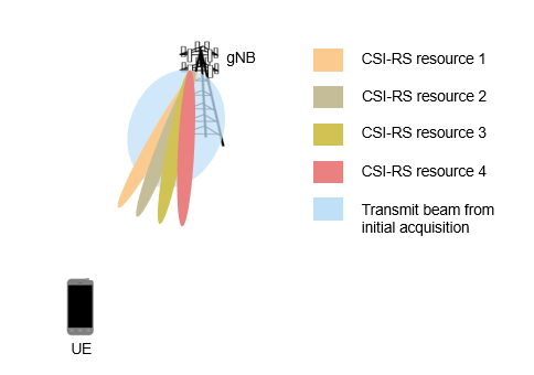
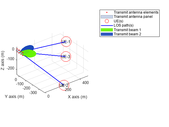
Plot Tx beamforming pattern. This plot displays the selected CSI-RS beam for a UE node with highest L1-RSRP and assigns each beam a unique beam index across the SSBs.
if enableBeamforming
    hPlotBeamformingPattern(simParameters, gNB, beamIndices);
end
Obtain the simulation metrics and save it in a MAT-file. The MAT-file 'simulationMetricsFile' saves the simulation metrics.
metrics = getMetrics(metricsVisualizer);
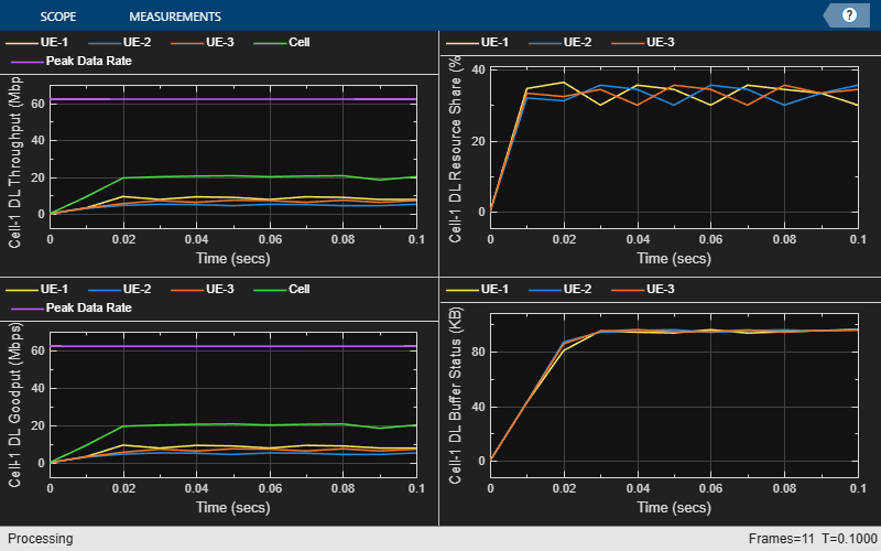
save(simulationMetricsFile,'metrics');At the end of the simulation, compare the achieved values for system performance indicators with theoretical peak values (considering zero overheads). Performance indicators displayed are achieved data rate (DL), achieved spectral efficiency (DL), and BLER observed for UEs (DL). The calculated peak values are in accordance with 3GPP TR 37.910. This example considers that the number of layers used for the peak DL data rate calculation equals the average value of the maximum layers possible for each UE node in the respective direction. The maximum number of DL layers possible for a UE node is minimum of its Rx antennas and gNB's Tx antennas.
displayPerformanceIndicators(metricsVisualizer);
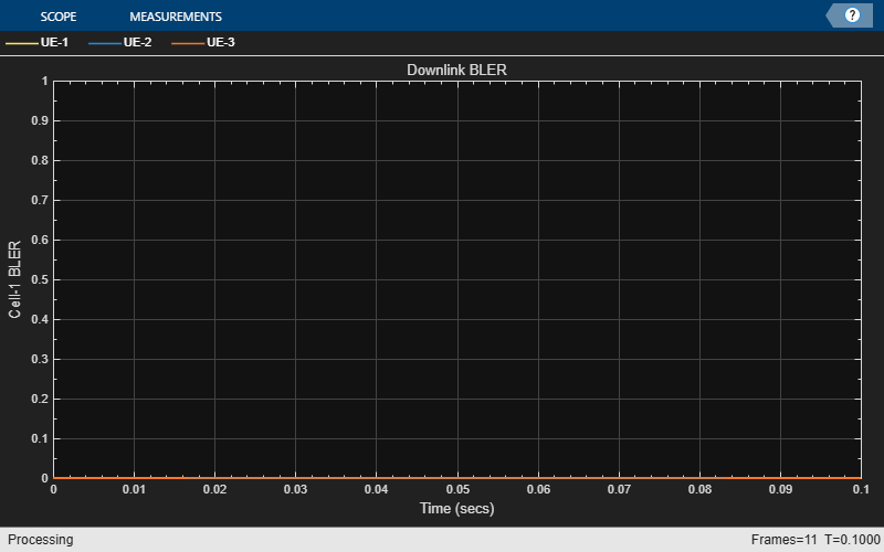
Peak DL Throughput: 62.21 Mbps. Achieved Cell DL Throughput: 18.96 Mbps
Achieved DL Throughput for each UE: [7.98        4.63        6.35]
Achieved Cell DL Goodput: 18.96 Mbps
Achieved DL Goodput for each UE: [7.98        4.63        6.35]
Peak DL spectral efficiency: 12.44 bits/s/Hz. Achieved DL spectral efficiency for cell: 3.79 bits/s/Hz

Block error rate for each UE in the downlink direction: [0  0  0]
The simulation results show the performance metrics with DL beamforming.
Simulation Visualization
The five types of run-time visualization shown are:
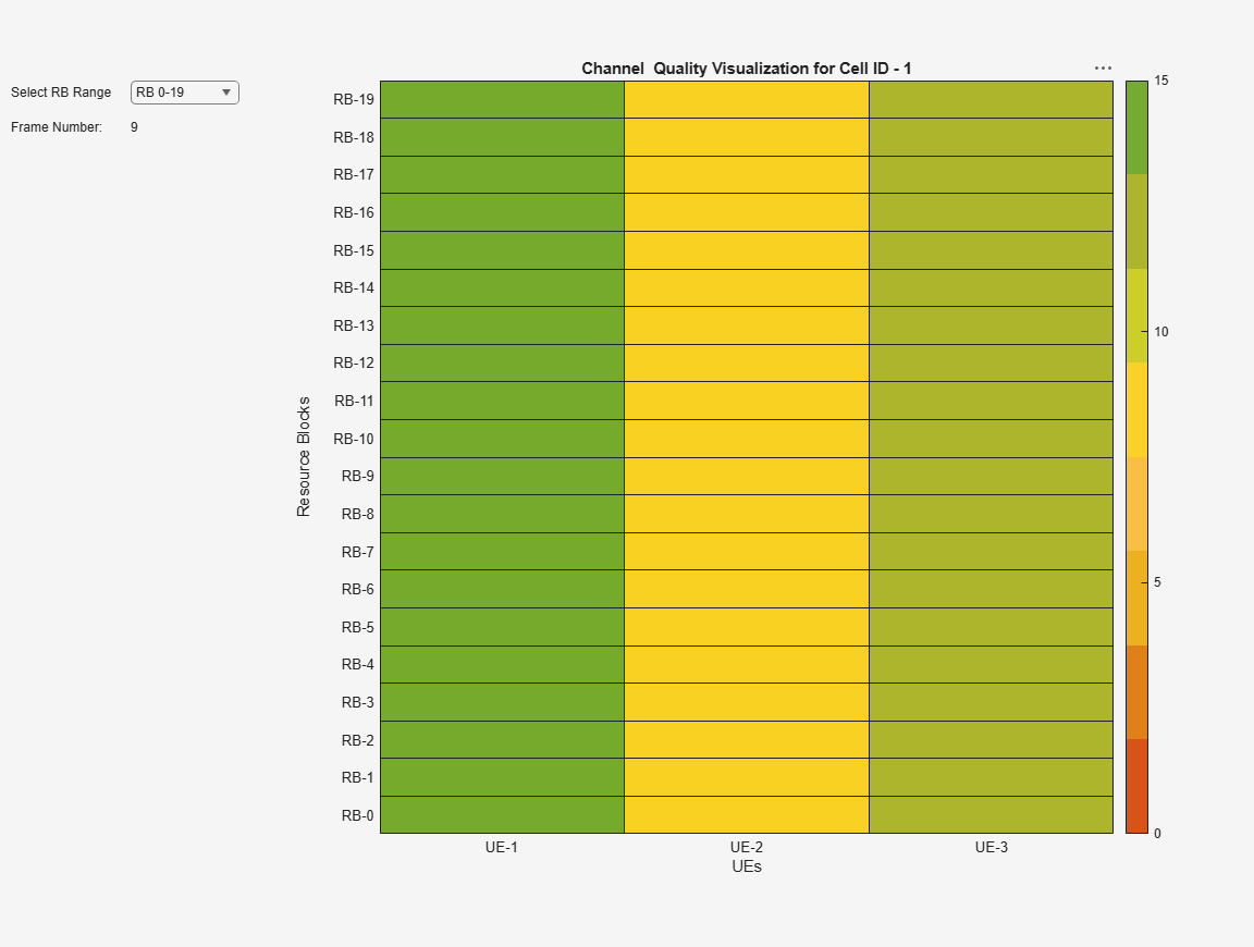
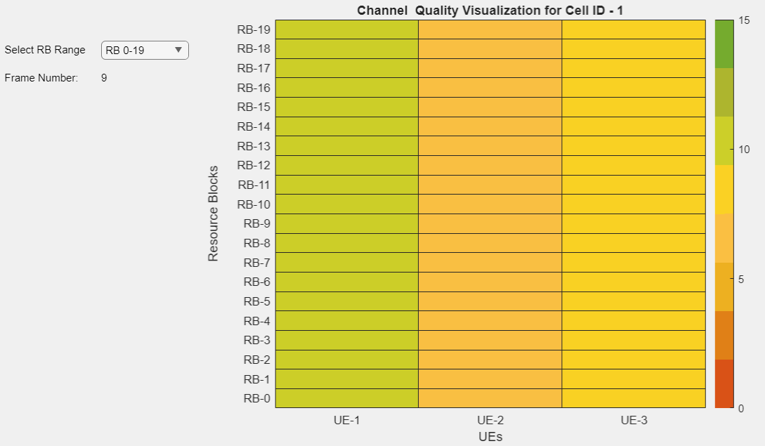
Display of CQI values for UEs over the channel bandwidth: For more information about this, see the 'Channel Quality Visualization' figure description in the NR Cell Performance Evaluation with Physical Layer Integration example.
Display of resource grid assignment to UEs: The 2D time-frequency grid shows the resource allocation to the UEs. You can enable this visualization in the 'Scenario Configuration' section. For more information about this, see the 'Resource Grid Allocation' figure description in the NR Cell Performance Evaluation with Physical Layer Integration example.
Display of DL scheduling metrics plots: For more information about this, see the 'Downlink Scheduler Performance Metrics ' figure description in the NR Cell Performance Evaluation with Physical Layer Integration example.
Display of DL Block Error Rates: For more information about this, see the 'Block Error Rate (BLER) Visualization' figure description in the NR Cell Performance Evaluation with Physical Layer Integration example.
Display of DL beamforming pattern: The figure shows the beam with highest L1-RSRP for each UE node. The gNB uses this beam directions for beamforming PDSCH and CSI-RS (for RI, CQI, PMI measurements) to the UEs. Two or more UE nodes can report same beam as its highest L1-RSRP beam.
Results With Beamforming Disabled
These are the simulation results when disabling DL beamforming. You can observe the network performance and CQI index for each UE.
For more information about the simulation logs, see the 'Simulation Logs' section in the NR Cell Performance Evaluation with Physical Layer Integration example.
if enableTraces
    simulationLogs = cell(1,1);
    if simParameters.DuplexMode == 0 % FDD
        logInfo = struct('DLTimeStepLogs',[],'SchedulingAssignmentLogs',[],'BLERLogs',[],'AvgBLERLogs',[]);
        [logInfo.DLTimeStepLogs,~] = getSchedulingLogs(simSchedulingLogger);
    else % TDD
        logInfo = struct('TimeStepLogs',[],'SchedulingAssignmentLogs',[], ...
            'BLERLogs',[],'AvgBLERLogs',[]);
        logInfo.TimeStepLogs = getSchedulingLogs(simSchedulingLogger);
    end
    % BLER logs
    [logInfo.BLERLogs,logInfo.AvgBLERLogs] = getBLERLogs(simPhyLogger);
    % Scheduling assignments log
    logInfo.SchedulingAssignmentLogs = getGrantLogs(simSchedulingLogger);
    simulationLogs{1} = logInfo;
    % Save simulation parameters in a MAT-file
    save(parametersLogFile,'simParameters');
    % Save simulation logs in a MAT-file
    save(simulationLogFile,'simulationLogs');
end
You can run the script NRPostSimVisualization to get a post-simulation visualization of logs. For more information about the options to run this script, refer to the NR Cell Performance Evaluation with Physical Layer Integration example.
Further Exploration
You can use this example to further explore custom scheduling.
Custom scheduling
You can modify the existing scheduling strategy to implement a custom one. Use Custom Scheduler in 5G System-Level Simulation example explains how to create a custom scheduling strategy and plug it into system-level simulation. MIMO configuration appends more fields to the scheduling assignment structure. Populate the fields of scheduling assignments with values for precoding matrix, number of layers, beamforming table index as per your custom scheduling strategy. The beamforming table index corresponds to the columns in the table 'simParameters.BeamWeightTable'. For more information about the information fields of a scheduling assignment, see the description of the scheduleDLResourcesSlot and scheduleULResourcesSlot functions in the hNRScheduler helper file.
Local functions
function ssbIndex = computeSSBToUE(simParameters,ssbTxAngles,ssbSweepRange,ueRelPosition)
%   SSBINDEX = computeSSBtoUE(SIMPARAMETERS,SSBTXANGLES,SSBSWEEPRANGE,UERELPOSITION)
%   computes an SSB to the UE node based on SSBTXANGLES and SSBSWEEPRANGE. If a UE
%   node falls within the sweep range of an SSB, then the function
%   assigns corresponding SSBINDEX.
%   If a UE node does not fall under any of the SSBs then the
%   function approximates the UE node to its nearest SSB.
ssbIndex = zeros(1,simParameters.NumUEs);
for i=1:simParameters.NumUEs
    if (ueRelPosition(i,2) > (ssbTxAngles(1) - ssbSweepRange/2)) && ...
            (ueRelPosition(i,2) <= (ssbTxAngles(1) + ssbSweepRange/2))
        ssbIndex(i) = 1;
    elseif (ueRelPosition(i,2) > (ssbTxAngles(2) - ssbSweepRange/2)) && ...
            (ueRelPosition(i,2) <= (ssbTxAngles(2) + ssbSweepRange/2))
        ssbIndex(i) = 2;
    elseif (ueRelPosition(i,2) > (ssbTxAngles(3) - ssbSweepRange/2)) && ...
            (ueRelPosition(i,2) <= (ssbTxAngles(3) + ssbSweepRange/2))
        ssbIndex(i) = 3;
    elseif (ueRelPosition(i,2) > (ssbTxAngles(4) - ssbSweepRange/2)) && ...
            (ueRelPosition(i,2) <= (ssbTxAngles(4) + ssbSweepRange/2))
        ssbIndex(i) = 4;
    else % Approximate the UE node to the nearest SSB
         % Initialize an array to store the difference between the UE azimuth and
         % SSB azimuth beam sweep angles
        angleDiff = zeros(1,length(ssbTxAngles));
        for angleIdx = 1: length(ssbTxAngles)
            angleDiff(angleIdx) = abs(ssbTxAngles(angleIdx) - ueRelPosition(i,2));
        end
         % Minimum azimuth angle difference
        [~,idx] = min(angleDiff);
        ssbIndex(i) = idx;
    end
end
end
Copyright 2021-2026 The MathWorks, Inc..
References
[1] 3GPP TS 38.214. “NR; Physical layer procedures for data.” 3rd Generation Partnership Project; Technical Specification Group Radio Access Network.
[2] 3GPP TS 38.321. “NR; Medium Access Control (MAC) protocol specification.” 3rd Generation Partnership Project; Technical Specification Group Radio Access Network.
[3] 3GPP TS 38.322. “NR; Radio Link Control (RLC) protocol specification.” 3rd Generation Partnership Project; Technical Specification Group Radio Access Network.
[4] 3GPP TR 38.901. “Study on channel model for frequencies from 0.5 to 100 GHz.” 3rd Generation Partnership Project; Technical Specification Group Radio Access Network.