NR Cell Performance with Downlink MU-MIMO
This example demonstrates how to evaluate the system performance of downlink (DL) multi-user (MU) multiple-input multiple-output (MIMO) using the 5G Toolbox™, with a focus on link-to-system mapping-based abstract physical layer (PHY).
Using this example, you can
Model downlink MU-MIMO.
Modify the MU-MIMO related scheduler configuration and observe the impact on cell performance.
Analyze cell performance for various channel delay profiles.
The simulation results focus on key performance indicators (KPIs) such as cell throughput, spectral efficiency, and block error rate (BLER).
Introduction
MU-MIMO is an important capability for increasing the capacity of a cellular network. Digital precoding facilitates MU-MIMO by spatially separating user transmissions over common time and frequency resources.
For DL MU-MIMO, a 5G NR base station (gNB) determines the precoder using one of these techniques:
The gNB uses reported channel state information (CSI) Type II precoders. For more information about this technique, see the 5G NR Downlink CSI Reporting example.
In a time division duplex (TDD) system, the gNB computes the DL precoder from the sounding reference signal (SRS) using channel reciprocity. For more information about this technique, see the TDD Reciprocity-Based PDSCH MU-MIMO Using SRS example.
In this example, the gNB facilitates DL MU-MIMO by using two approaches: CSI Type II precoding and SRS-based precoding in TDD systems.
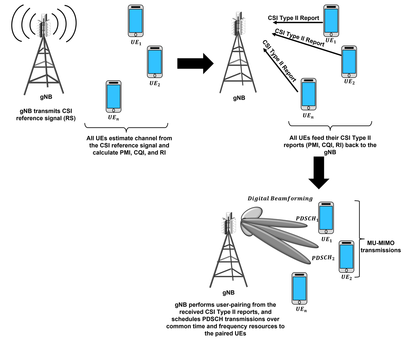
CSI-RS-Based DL MU-MIMO
This overview details the communication process between the gNB and user equipment (UE) nodes in a CSI-RS-based DL MU-MIMO system.
The gNB transmits the CSI reference signal (CSI-RS).
UE nodes in the same cell estimate the channel from the CSI-RS.
Each UE determines a rank indicator (RI), precoder matrix indicator (PMI), and channel quality indicator (CQI) from the estimated channel.
UE nodes report RI, PMI, and CQI to the gNB.
The CSI reported by the UE forms the basis for the DL user-pairing algorithm.
For paired UE nodes, the gNB node transmits precoded DL signals over shared time and frequency resources.
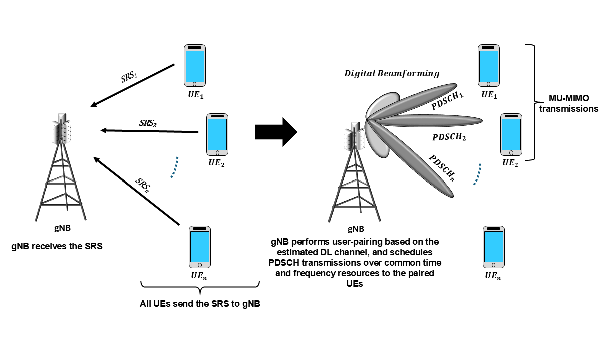
SRS-Based DL MU-MIMO in TDD Systems
This overview details the communication flow between UE and gNB nodes in a SRS-based DL MU-MIMO system.
The UE nodes transmit the SRS.
The gNB estimates the uplink (UL) channel from the received SRS.
Using channel reciprocity, the gNB node directly estimates the DL channel from the SRS.
The gNB uses channel estimations from all UE nodes to drive the DL user-pairing algorithm.
For paired UE nodes, the gNB node transmits precoded DL signals over shared time and frequency resources.
For more information about UL CSI estimation by using SRS, see the NR Uplink Channel State Information Estimation Using SRS example.
Simulation Assumptions
This example makes these assumptions.
The number of CSI-RS ports equals the number of transmit antennas on the gNB.
The number of SRS antenna ports equals the number transmit antennas of the UE node.
The scheduler pairs only UE nodes that report the same rank in case of CSI-RS-based MU-MIMO. Therefore, the scheduler does not pair two UE nodes if one of the UE nodes report a rank of
1and the other UE reports a rank of2.The gNB transmits retransmission packets as a single-user (SU) MIMO.
In this example, the scheduler does not support effective Modulation and Coding Scheme (MCS) calculation for paired UE nodes in CSI-RS-based DL MU-MIMO. Instead, it uses the MCS corresponding to the Channel Quality Indicator (CQI) reported by the UE nodes, which can lead to a higher BLER, especially when you set the SemiOrthogonalityFactor to a value less than 1. For SRS-based DL MU-MIMO, the scheduler recomputes the effective MCS and precoding matrices for paired UE nodes. However, it does not perform rank selection as part of pairing; the UE nodes will use the selected ranks based on the single-User MIMO setting.
The scheduler uses
SemiOrthogonalityFactorand the reported PMI indices (i1) for user-pairing in case of CSI-RS-based MU-MIMO.The scheduler uses wideband DL channel estimates from the SRS measurements for user-pairing in case of SRS-based MU-MIMO.
Simulate Scenario
Create a wireless network simulator.
rng("default") % Reset the random number generator numFrameSimulation =50; % Simulation time in terms of number of 10 ms frames networkSimulator = wirelessNetworkSimulator.init;
Set duplexType to "TDD" or "FDD". For SRS-based DL MU-MIMO, you must set duplexType to "TDD".
duplexType =  "TDD";
Create a gNB node and specify these parameters.
Transmit power — 34 dBm
Subcarrier spacing — 15 kHz
Carrier frequency — 2.6 GHz
Channel bandwidth — 5 MHz
Number of transmit antennas — 32
Number of receive antennas — 32
Duplex mode — TDD
Receive gain — 11 dB
SRS transmission periodicity for all UE nodes connecting to this gNB — 20 slots
gNBPosition = [0 0 30]; % [x y z] meters position in Cartesian coordinates
gNB = nrGNB(Name="gNB", Position=gNBPosition, TransmitPower=34, SubcarrierSpacing=15000, ...
    CarrierFrequency=2.6e9, ChannelBandwidth=5e6, NumTransmitAntennas=32, ...
    NumReceiveAntennas=32, DuplexMode=duplexType, ReceiveGain=11, ...
    SRSPeriodicityUE=20, NumResourceBlocks=25);
Set the downlink CSI measurement signal type, csiMeasurementSignalDLType, to "SRS". Alternatively, you can set it to "CSI-RS". Note that the user-pairing algorithm depends on the selected type of downlink measurement signal.
csiMeasurementSignalDLType =  "SRS";
Configure the DL MU-MIMO structure muMIMOConfiguration by setting these fields. For more information about these fields, see the MUMIMOConfigDL name-value argument of configureScheduler function.
Maximum number of UE nodes paired — 2
Maximum number of layers — 8
Minimum number of RBs — 2
Minimum DL SINR — 10 dB
muMIMOConfiguration = struct(MaxNumUsersPaired=2, MaxNumLayers=8, MinNumRBs=2, ...
    MinSINR=10);
Set these scheduler parameters by using the configureScheduler function.
Resource allocation type — 0
Maximum number of UE nodes per transmission time interval (TTI) — 10
MU-MIMO configuration structure —
muMIMOConfigurationCSI measurement signal for DL — SRS
allocationType =0; % Resource allocation type configureScheduler(gNB, ResourceAllocationType=allocationType, ... MaxNumUsersPerTTI=10, MUMIMOConfigDL=muMIMOConfiguration, ... CSIMeasurementSignalDL=csiMeasurementSignalDLType);
Set the number of UE nodes, and compute positions of all UE nodes using these specifications.
Relative distance of the UE from the gNB —
500(Units are in meters)Sweep range of the azimuth angle in the horizontal plane —
[-60 60](Units are in degrees)
numUEs =10; % Number of UE nodes
% For all UEs, specify position in spherical coordinates (r, azimuth, elevation)
% relative to gNB.
ueRelPosition = [ones(numUEs, 1)*500 (rand(numUEs, 1)-0.5)*120 zeros(numUEs, 1)];
% Convert spherical to Cartesian coordinates considering gNB position as origin
[xPos, yPos, zPos] = sph2cart(deg2rad(ueRelPosition(:,2)), ...
    deg2rad(ueRelPosition(:,3)), ueRelPosition(:,1));
% Convert to absolute Cartesian coordinates
uePositions = [xPos yPos zPos] + gNBPosition;
ueNames = "UE-" + (1:size(uePositions,1));
Create the UE nodes. Specify the name, position, receiver gain, number of transmit antennas, and number of receive antennas for each UE.
UEs = nrUE(Name=ueNames, Position=uePositions, ReceiveGain=0, ...
    NumTransmitAntennas=1, NumReceiveAntennas=1);
Connect the UEs to the gNB and configure full-buffer traffic in the DL direction. Specify the CSI report periodicity (in slots).
connectUE(gNB, UEs, FullBufferTraffic="DL", CSIReportPeriodicity=10)Add the gNB and UE nodes to the network simulator.
addNodes(networkSimulator, gNB)
addNodes(networkSimulator, UEs)
Create an N-by-N matrix of link-level channels. N is the number of nodes in the cell. An element at index (i, j) contains the channel instance from node i to node j. An empty element at index (i, j) indicates that channel from node i to node j does not exist. i and j denote the node IDs.
% Set delay profile, delay spread (in seconds), and maximum Doppler
% shift (in Hz)
channelConfig = struct(DelayProfile="CDL-C", DelaySpread=10e-9, ...
    MaximumDopplerShift=1);
channels = hNRCreateCDLChannels(channelConfig, gNB, UEs);
Create a custom channel model using channels. Install the custom channel on the simulator. The network simulator applies the channel for a packet in transit before passing the packet to the receiver.
customChannelModel  = hNRCustomChannelModel(channels);
addChannelModel(networkSimulator, @customChannelModel.applyChannelModel)
Set enableTraces to true to log the traces. If you set enableTraces to false, the simulator does not log traces. Setting enableTraces to false can speed up your simulation.
enableTraces =  true;
true;Set up the scheduling logger and PHY logger.
if enableTraces
    % Create an object for scheduler trace logging
    simSchedulingLogger = helperNRSchedulingLogger(numFrameSimulation, gNB, UEs);
    % Create an object for PHY trace logging
    simPhyLogger = helperNRPhyLogger(numFrameSimulation, gNB, UEs);
end
Specify the number of metric plot updates per second, numMetricPlotUpdates, during the simulation.
% This parameter impacts the simulation time
numMetricPlotUpdates =200;
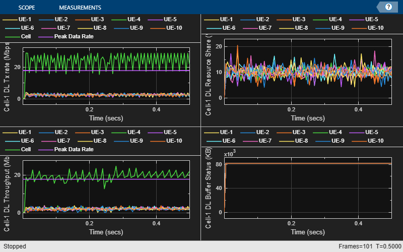
Set up a metric visualizer.
metricsVisualizer = helperNRMetricsVisualizer(gNB, UEs, ...
    RefreshRate=numMetricPlotUpdates, PlotSchedulerMetrics=true, ...
    PlotPhyMetrics=false,PlotCDFMetrics=true,LinkDirection="DL");
Write the logs to a MAT file. You can use these logs for post-simulation analysis.
if enableTraces
    simulationLogFile = "simulationLogs"; % For logging the simulation traces
end
Display the network topology.
networkVisualizer = wirelessNetworkViewer(ShowNodeNames=false);
addNodes(networkVisualizer, gNB)
addNodes(networkVisualizer, UEs)
Run the simulation for the specified number of frames numFrameSimulation.
% Calculate the simulation duration (in seconds)
simulationTime = numFrameSimulation*1e-2;
% Run the simulation
run(networkSimulator, simulationTime);
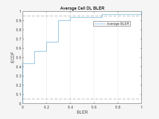
Results Summary
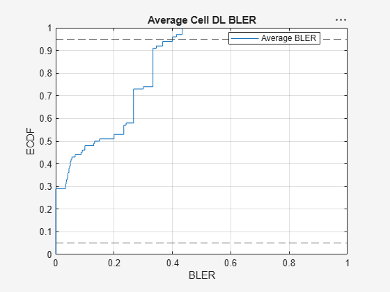
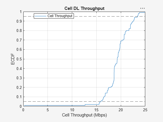
Display the system KPIs, including cell throughput, spectral efficiency and, empirical cumulative distribution function (ECDF) plots for cell throughput and average BLER. Using the ECDF plots, you can find the proportion of slots in which the throughput and BLER are less than or equal to specific values indicated on the x-axis.
% Read performance metrics
displayPerformanceIndicators(metricsVisualizer)
Peak DL throughput: 17.77 Mbps Achieved cell DL throughput: 19.28 Mbps Achieved DL throughput for each UE: [1.95 2.02 1.93 2 1.9 1.94 1.93 1.94 1.83 1.83] Peak DL spectral efficiency: 3.55 bits/s/Hz Achieved DL spectral efficiency for cell: 3.86 bits/s/Hz Block error rate for each UE in the DL direction: [0.16 0.165 0.162 0.163 0.181 0.163 0.188 0.181 0.22 0.204]
Block error rate (BLER) can arise from multiple factors, including situations where the actual resource overhead in a slot, such as from CSI-RS transmissions, exceeds the overhead value (xOH) used in the transport block size (TBS) calculation. According to 3GPP TS 38.214, section 5.1.3.2, xOH has a maximum value of 18, even when the number of CSI-RS ports is set to 32. When the gNB configures 32 ports, the real overhead can exceed the xOH value, leading to increased rate matching puncturing and assured packet decode failure when PDSCH and CSI-RS share the same slot.
if enableTraces
    simulationLogs = cell(1, 1);
    if gNB.DuplexMode == "FDD"
        logInfo = struct(DLTimeStepLogs=[], ULTimeStepLogs=[], ...
            SchedulingAssignmentLogs=[], PhyReceptionLogs=[]);
        [logInfo.DLTimeStepLogs, logInfo.ULTimeStepLogs] = ...
            getSchedulingLogs(simSchedulingLogger);
    else % TDD
        logInfo = struct(TimeStepLogs=[], SchedulingAssignmentLogs=[], ...
            PhyReceptionLogs=[]);
        logInfo.TimeStepLogs = getSchedulingLogs(simSchedulingLogger);
    end
    % Get the scheduling assignments log
    logInfo.SchedulingAssignmentLogs = getGrantLogs(simSchedulingLogger);
    % Get the PHY reception logs
    logInfo.PhyReceptionLogs = getReceptionLogs(simPhyLogger);
    % Save simulation logs in a MAT-file
    simulationLogs{1} = logInfo;
    save(simulationLogFile, "simulationLogs")
end
Display a histogram of the average number of UE nodes per RB per DL slot, indicating the average number of UE nodes assigned to the same RB in each DL transmission slot. The calculation of this metric follows the distinct frequency allocation methods used in resource allocation types 0 and 1.
RAT0
Average number of UE nodes per RB (slot)
is the total number of Resource Block Groups (RBGs).
is the number of UE nodes assigned to the i-th RBG.
is the number of RBs in the i-th RBG.
is the total number of RBs in the carrier bandwidth.
RAT1
Average number of UE nodes per RB (slot)
is the total number of Resource Blocks (RBs).
is the number of UE nodes assigned to the j-th RB.
is the total number of RBs in the carrier bandwidth.
if enableTraces
    avgNumUEsPerRB = calculateAvgUEsPerRBDL(logInfo, gNB.NumResourceBlocks, allocationType, duplexType);
    % Plotting the histogram
    figure
    theme("light")
    histogram(avgNumUEsPerRB, "BinWidth", 0.1);
    title("Distribution of Average Number of UEs per RB in DL Slots");
    xlabel("Average Number of UEs per RB");
    ylabel("Number of Occurrence");
    grid on
end
This histogram shows the level of pairing among UE nodes, indicating how frequently multiple users share the same resource block in MU-MIMO transmission.
Local Function
Calculate the average number of UE nodes per RB per DL slot and visualize this metric to get an indication of level of user-pairing.
function avgUEsPerRB = calculateAvgUEsPerRBDL(logInfo, numResourceBlocks, ratType, duplexMode)
    %calculateAvgUEsPerRBDL Calculate average number of UE nodes per RB in DL slots.
    %   AVGUESPERRB = calculateAvgUEsPerRBDL(LOGINFO, NUMRESOURCEBLOCKS, RATTYPE,
    %   DUPLEXMODE) calculates the average number of UE nodes per RB for each DL
    %   slot based on the log information.
    %
    %   LOGINFO is a structure containing detailed logs of the simulation.
    %   NUMRESOURCEBLOCKS is an integer specifying the number of resource blocks in
    %   carrier bandwidth RATTYPE is an integer indicating the resource allocation
    %   type (0 or 1). DUPLEXMODE is a string that indicates the duplex mode, which
    %   can be either "TDD" or "FDD".
    %
    %   The function returns AVGUEsPerRB, a vector containing the average number of
    %   UE nodes per RB for each DL slot, allowing for analysis of resource
    %   allocation efficiency.

    % Determine the appropriate data source based on the duplex mode
    if strcmp(duplexMode, "TDD")
        timeStepLogs = logInfo.TimeStepLogs;
        freqAllocations = timeStepLogs(:, 5);
    elseif strcmp(duplexMode, "FDD")
        timeStepLogs = logInfo.DLTimeStepLogs;
        freqAllocations = timeStepLogs(:, 4);
    end

    % Extract the number of slots
    numOfSlots = size(timeStepLogs, 1) - 1;

    % Determine RBG sizes for RAT0
    if ~ratType
        % Determine the nominal RBG size P based on TR 38.214
        numRBG = size(freqAllocations{2}, 2);
        P = ceil(numResourceBlocks / numRBG);
        % Initialize the RBG sizes
        numRBsPerRBG = P * ones(1, numRBG);
        % Calculate the size of the last RBG
        remainder = mod(numResourceBlocks, P);
        if remainder > 0
            numRBsPerRBG(end) = remainder;
        end
    end

    % Initialize a vector to store the average number of UEs per RB for DL slots
    avgUEsPerRB = zeros(1, numOfSlots);

    % Iterate over each slot
    for slotIdx = 1:numOfSlots
        % For TDD, extract the type of slot (DL or UL)
        if strcmp(duplexMode, "TDD")
            slotType = timeStepLogs{slotIdx + 1, 4};
            if ~strcmp(slotType, "DL")
                continue; % Skip UL slots in TDD
            end
        end

        % Extract the frequency allocation for the current DL slot
        freqAllocation = freqAllocations{slotIdx + 1};

        if ~ratType
            % Process RAT0
            totalUniqueUEs = sum(arrayfun(@(rbgIdx) nnz(freqAllocation(:, rbgIdx) > 0) * ...
                numRBsPerRBG(rbgIdx), 1:length(numRBsPerRBG)));
            avgUEsPerRB(slotIdx) = totalUniqueUEs / numResourceBlocks;

        else
            % Process RAT1
            ueRBUsage = zeros(1, numResourceBlocks); % Vector to count UEs per RB

            for ueIdx = 1:size(freqAllocation, 1)
                startRB = freqAllocation(ueIdx, 1);
                numContiguousRBs = freqAllocation(ueIdx, 2);
                ueRBUsage(startRB + 1:(startRB + numContiguousRBs)) = ...
                    ueRBUsage(startRB + 1:(startRB + numContiguousRBs)) + 1;
            end

            avgUEsPerRB(slotIdx) = mean(ueRBUsage(ueRBUsage > 0));
        end
    end

    % Remove entries for UL slots (if any), which is relevant for TDD
    avgUEsPerRB = avgUEsPerRB(avgUEsPerRB > 0);
end
Further Explorations
Try running the example with these modifications.
Analyze the impact of various CDL delay profiles (CDL-A/B/C/D/E) on the user-pairing strategy and system KPIs.
Analyze the impact of antenna configurations, such as CSI antenna ports, panel configuration, antenna orientation, and channel delay profile, on the system KPIs.
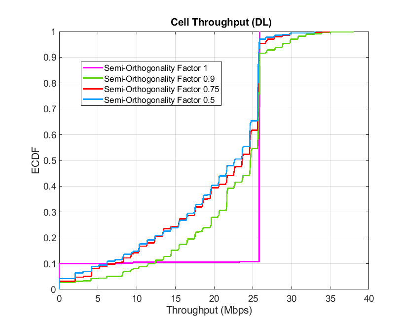
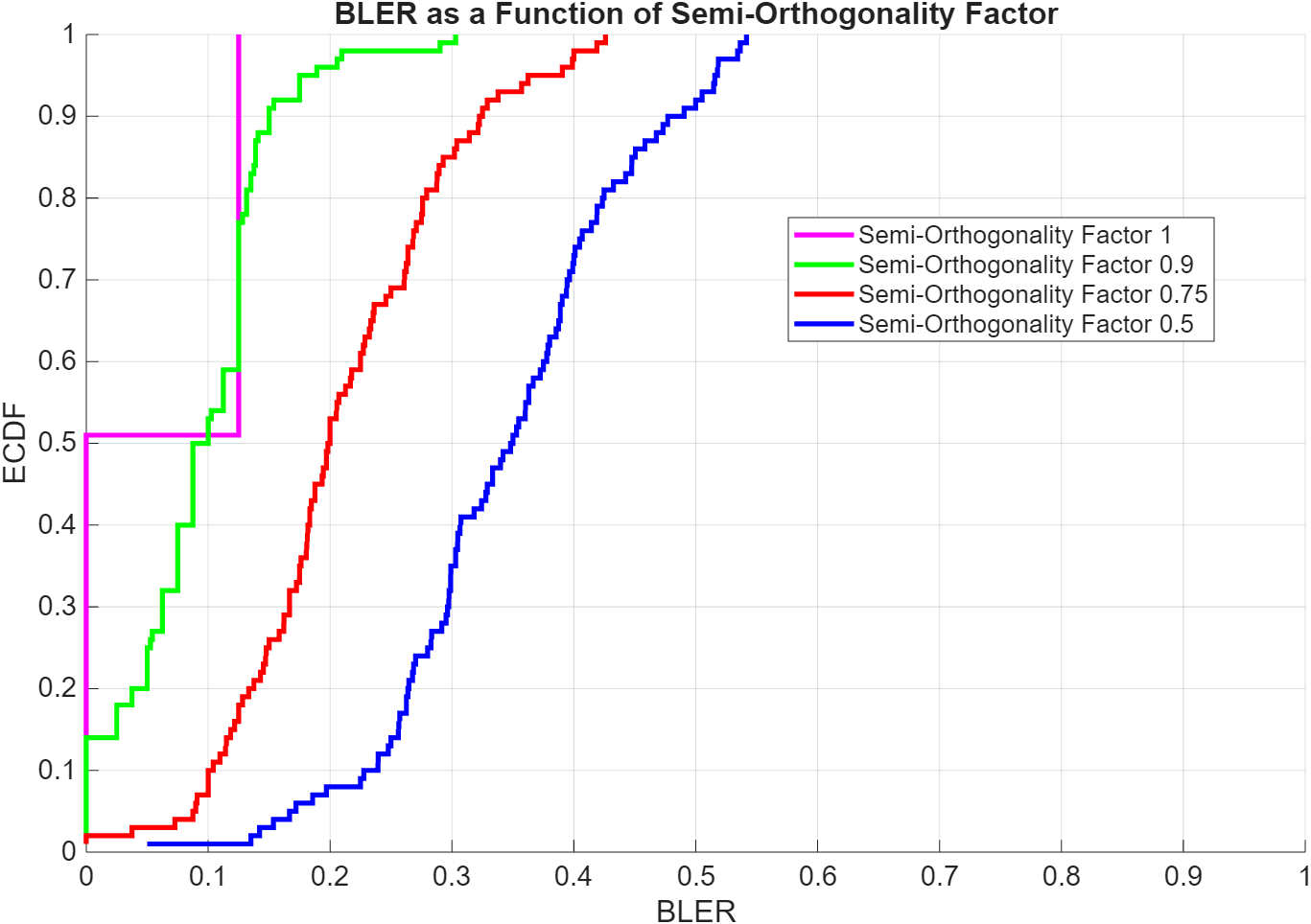
Modify the DL MU-MIMO configuration and observe its impact on the system KPIs. For example, this table shows the relationship between
SemiOrthogonalityFactorand average BLER for a static scenario with 40 UE nodes in frequency division duplex (FDD) mode.This simulation setup does not compute the effective MCS when the scheduler pairs users for CSI-RS-based DL MU-MIMO.
Semi-Orthogonality Factor | Average BLER |
1.0 | 0.0982 |
0.9 | 0.1255 |
0.75 | 0.2387 |
0.5 | 0.3712 |
These figures illustrate the impact of the SemiOrthogonalityFactor on average BLER and cell throughput. For the considered scenario with FDD mode, orthogonal users do not exist when you set SemiOrthogonalityFactor to 1 and use CSI Type II precoder.

Modify the DL CSI measurement signal type and observe its impact on the MU-MIMO performance. For example, these plots show the average BLER and cell throughput comparison for CSI-RS and SRS-based SU-MIMO and MU-MIMO in the TDD mode.


Supporting Functions
The example uses these helper classes and functions:
helperNRMetricsVisualizer– Implements metrics visualization functionalityhelperNRSchedulingLogger– Implements scheduling information logging functionalityhelperNRPhyLogger– Implements PHY packet reception information logging functionalityhNRCreateCDLChannels– Creates CDL channels for gNB-to-UE and UE-to-gNB linkshNRCustomChannelModel– Implements channel modeling functionalityhNRKPIManager: Implements functionality for calculating key performance indicators
Copyright 2022-2026 The MathWorks, Inc..
References
[1] 3GPP TS 38.214. “NR; Physical layer procedures for data.” 3rd Generation Partnership Project; Technical Specification Group Radio Access Network.
See Also
Objects
wirelessNetworkSimulator(Wireless Network Toolbox) |nrGNB|nrUE