Run 5G System-Level Simulations on AWS Cloud

Overview

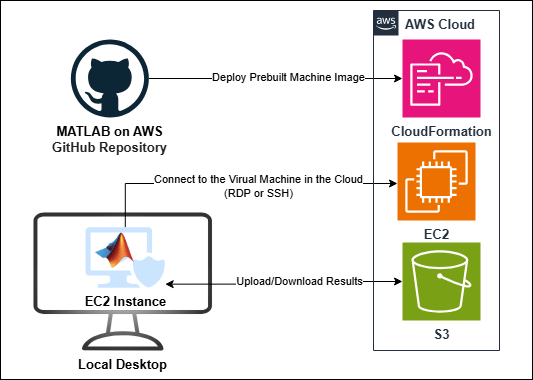
The MATLAB on AWS architecture enables you to deploy MATLAB on an Amazon Elastic Compute Cloud (EC2) instance using your AWS account, and connect to the EC2 instance using remote desktop protocol (RDP) or secure shell (SSH). This architecture also integrates with AWS storage services, such as the Amazon Simple Storage Service (S3). You can store data and simulation results in Amazon S3, enabling you to easily transfer files between AWS and your local desktop. Your local desktop serves as the MATLAB user interface, while AWS provides scalable compute power and storage, creating a flexible and cost-effective environment for cloud-based MATLAB simulations. The architecture uses an AWS CloudFormation template from the MATLAB on AWS GitHub repository for automation.

Use the MATLAB on AWS architecture when you need to:

You can select from a range of AWS EC2 instance types to meet your performance requirements and budget. The AWS EC2 service provides a secure and efficient setup for running MATLAB, supports multiple licensing options, and offers seamless storage integration.

AWS Services and Costs

This example uses these AWS services:

You are responsible for the cost of the AWS services used when you create cloud resources using this guide. Resource settings, such as instance type, affect the cost of deployment. For cost estimates, see the pricing pages for each AWS service you are using. Prices are subject to change. You can visualize, understand, and manage AWS costs and usage over time using AWS Cost Explorer.

Requirements for Using MATLAB Reference Architecture on AWS

To use the MATLAB on AWS architecture, make sure you have:

How to Run MATLAB on AWS

To run MATLAB on AWS, choose one of the these options:

Run MATLAB Using Prebuilt Amazon Machine Image from GitHub

By default, the MATLAB on AWS architecture launches a prebuilt machine image. Using a prebuilt machine image is a simple way to deploy MATLAB on AWS. Follow these steps to launch MATLAB on AWS.

Install MATLAB on Existing EC2 Instance

If you already have a running EC2 instance, you can manually install MATLAB by following these steps:

Run 5G System-Level Simulations

After starting MATLAB on your AWS instance, use 5G Toolbox™ to run 5G simulations. Running these models on AWS provides the scalability and performance required for large or complex workloads.

For hands-on experience, try running the NR Interference Modeling with Toroidal Wrap-Around example available in 5G Toolbox.

To open the example in MATLAB, copy this command to the MATLAB command line, uncomment and run it:

%openExample("5g/NRInterferenceModelingWithToroidalWrapAroundExample");

When running this example with a full PHY configuration and a large network, such as 19 cell sites, each with 3 sectors, and 20 UEs per cell, the memory requirements can reach several hundred gigabytes. This exceeds the capacity of most desktop systems, which typically provide limited RAM. Using cloud resources, such as AWS EC2 instances like r5.8xlarge that offer 256 GB or more of RAM, makes running such large-scale simulations feasible.

To accelerate computations such as TR 38.901 channel filtering and MIMO processing, you can enable GPU acceleration using Parallel Computing Toolbox. For example, AWS EC2 instances like g5.8xlarge (with NVIDIA® A10G GPUs) or p4d (with NVIDIA A100 GPUs) provide the necessary hardware for high-performance simulations.

In the example script, you can modify parameters such as the number of cell sites, number of sectors, number of UEs, antenna configurations, and wrap around. After adjusting these settings, run the simulation to analyze system-level performance.

Parameter Sweep for BLER Using Parallel Computing Toolbox

In 5G SLS, you often need to evaluate block error rate (BLER) across a range of conditions, such as different signal-to-interference-plus-noise ratio (SINR) values and modulation and coding scheme (MCS) indices. Running these simulations sequentially can take a long time because each configuration requires a separate run.

Use Parallel Computing Toolbox to run multiple simulations concurrently on separate cores. This approach is useful for:

These workloads often exceed the capabilities of a local desktop, which typically has limited memory and cores. For large-scale sweeps or full PHY simulations, AWS provides high-memory EC2 instances and GPU-enabled instances for PHY acceleration.

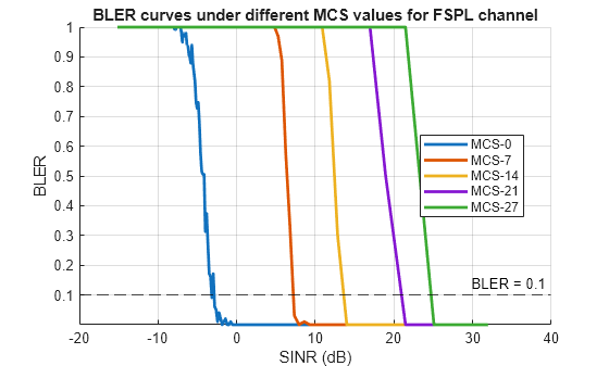
This example reproduces BLER curves using the free space path loss (FSPL) channel with an abstract PHY model. The figure shows the BLER versus SINR results obtained with the number of frames numFrames set to 100. You can produce similar results by adjusting numFrames in the example script.

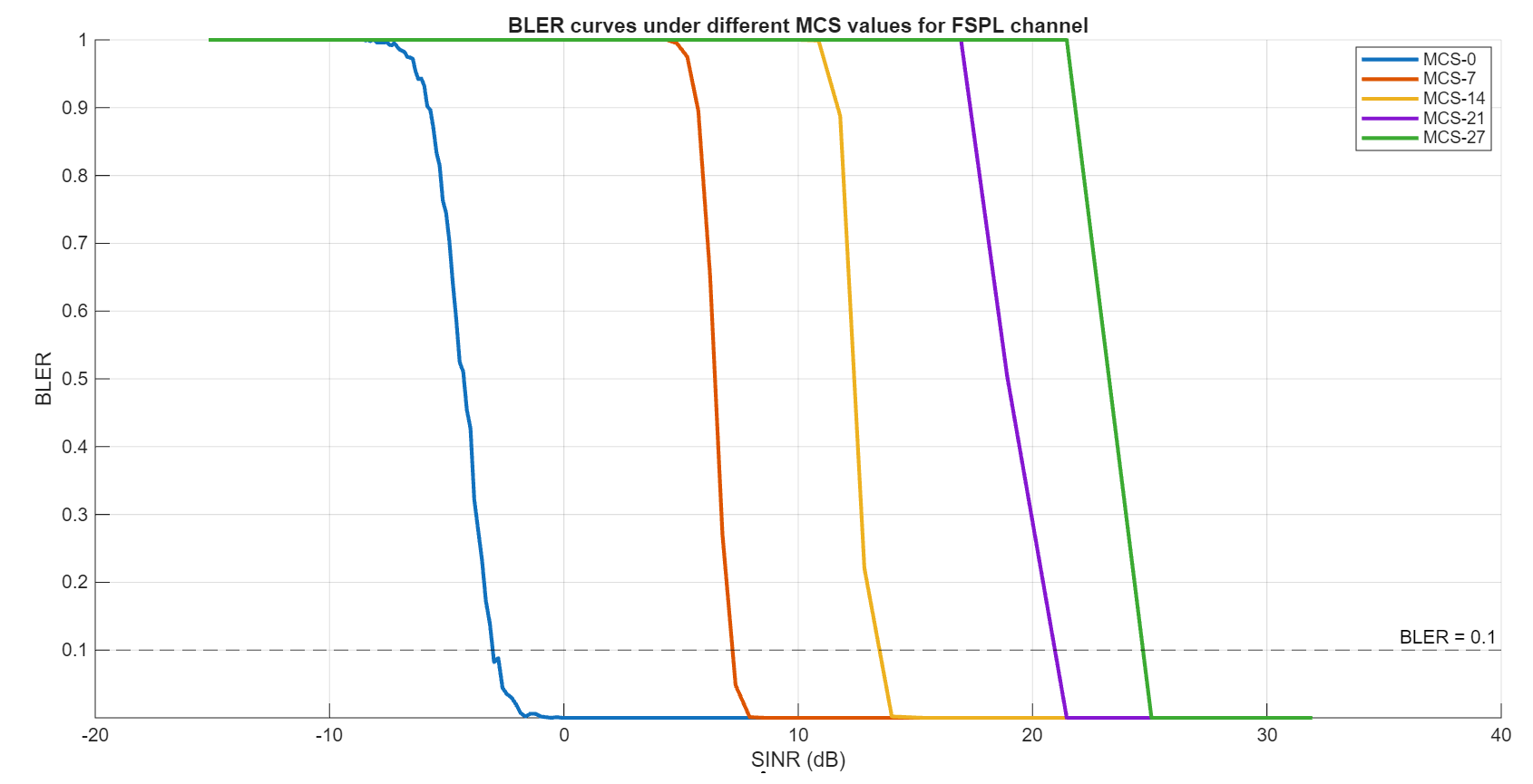
%%Parameter Sweep Simulation for BLER vs SINR
% This script demonstrates how to perform a parameter sweep using parallel
% simulations. It evaluates the BLER as a function of SINR for different
% MCS indices in a 5G scenario.
%
% The script also compares the execution time of parallel and serial
% simulations for the parameter sweep.

% Initialize parameters
mcsList = [0; 7; 14; 21; 27]; % From 3GPP TS 38.214, table 5.1.3.1-2: MCS Index table 2 for PDSCH
numFrames = 10;               % Simulation time in terms of number of frames
numUEs = 200;                 % Number of UEs in simulation
ueDistance = 300;             % The distance between UEs in meters

% Collect per-MCS BLER/SINR vectors in parallel
nMCS = numel(mcsList);
blerPar = cell(nMCS,1);
sinrPar = cell(nMCS,1);

% The parfor loop uses the Parallel Computing Toolbox to run
% simulations in parallel. If this toolbox is not available, the
% simulations execute serially.
tPar = tic;
parfor i = 1:nMCS
    mcsValue = mcsList(i);
    eventsFileName = "eventlogs_" + i;
    [bVals,sVals] = simulate5GDownlinkMCS(mcsValue,numFrames,numUEs,ueDistance,eventsFileName);

    % Store column vectors
    blerPar{i} = bVals(:);
    sinrPar{i} = sVals(:);
end
tPar = toc(tPar);

% Plot BLER vs SINR using parallel results
figure
hold on
grid on
colors = lines(nMCS);
epsBLER = 1e-6; % Minimum value to avoid zeros on log scale
for i = 1:nMCS
    sinrValues = sinrPar{i};
    blerValues = blerPar{i};
    blerValues = max(blerValues,epsBLER);  % Avoid zeros on log scale
    semilogy(sinrValues,blerValues,'-',Color=colors(i,:),LineWidth=2);
end

yline(0.1, "--k","BLER = 0.1")
xlabel("SINR (dB)")
ylabel("BLER")
ylim([epsBLER 1])
title("BLER curves under different MCS values for FSPL channel")
legend(arrayfun(@(x) sprintf("MCS-%d",x),mcsList,UniformOutput=false),Location="best")

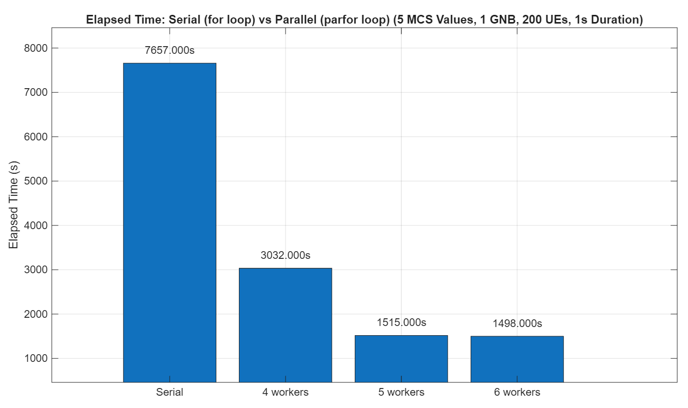
This figure shows the elapsed time taken to complete the simulations when run serially (for loop) and in parallel (parfor loop). Parallel execution significantly reduces the runtime for large parameter sweeps or Monte Carlo simulations. This example runs five parallel simulations, using up to five workers. Running a larger number of parallel simulations benefits from additional CPU cores. Cloud services such as AWS provide the necessary resources for such scalability.

Upload or Download Simulation Results

After running your 5G SLS in MATLAB, you can save the results to Amazon S3 for secure, persistent storage. This enables you to access your data even after your EC2 instance has stopped or been terminated.

To upload results from your EC2 instance to S3, uncomment and run this code, replacing /home/ubuntu/folder with your local directory path and s3://your-s3-bucket/folder with the path to your S3 bucket and folder:

% !aws s3 cp /home/ubuntu/folder s3://your-s3-bucket/folder --recursive

To download results from your S3 to EC2 instance, uncomment and run this code, replacing /home/ubuntu/folder with your local directory path and s3://your-s3-bucket/folder with the path to your S3 bucket and folder:

% !aws s3 cp s3://your-s3-bucket/folder /home/ubuntu/folder --recursive

Note: Replace /home/ubuntu/folder with your local directory path, and s3://your-s3-bucket/folder with your actual S3 bucket and folder path.

Your results remain securely stored in S3, so you can access or download them at any time. This ensures persistent storage and makes sharing or post-processing easy.

Delete Your Cloud Resources

Once you finish using your stack, delete all resources to avoid additional costs. To delete the stack, follow these steps:

Local Functions

function [blerVals,sinrVals] = simulate5GDownlinkMCS(mcsValue,numFrames,numUEs,ueDistance,fName)
%simulate5GDownlinkMCS Simulate a downlink 5G scenario for a fixed MCS
%   Runs a simple downlink (DL) only 5G network simulation. The scheduler
%   configures a fixed DL MCS without retransmission. This function
%   returns per-UE BLER and average SINR over the physical downlink shared
%   channel (PDSCH) receptions.

% Initialize network simulator
networkSimulator = wirelessNetworkSimulator.init;

% Create gNB object with specified parameters
gNB = nrGNB(Position=[30 0 30],ReceiveGain=0,TransmitPower=29,DuplexMode="FDD", ...
    ChannelBandwidth=50e6,SubcarrierSpacing=15e3,SRSPeriodicityUE=2560,NumResourceBlocks=200);

% Configure scheduler with fixed MCS and no retransmission. The value of
% RVSequence is a scalar for this reason.
configureScheduler(gNB,FixedMCSIndexDL=mcsValue,RVSequence=0,MaxNumUsersPerTTI=numUEs)

% Generate UE positions along the x-axis and create UE objects. Place UEs
% on a line starting at x = 10 m, spaced by ueDistance (m), keeping y and z
% coordinates at 0.
positions = zeros(numUEs,3);
xPositions = 10 + (0:(numUEs-1))*ueDistance;
positions(:, 1) = xPositions(:);

% Create nrUE objects with the specified parameters
ues = nrUE(Position=positions,ReceiveGain=0,TransmitPower=18);

% Connect UEs to gNB
connectUE(gNB,ues,FullBufferTraffic="DL")

% Add nodes to the network simulator
addNodes(networkSimulator,gNB)
addNodes(networkSimulator,ues)

% Add event tracer to log ReceptionEnded events to compute SINR
eventLogger = wirelessNetworkEventTracer(FileName=fName);
addNodes(eventLogger,ues,EventName="ReceptionEnded")

% Run the simulator
run(networkSimulator,numFrames*1e-2)

% Extract PHY metrics and compute BLER per UE
ueStats = statistics(ues);
phyStats = [ueStats.PHY];
nFailDL = [phyStats.DecodeFailures];
nPktDL = [phyStats.ReceivedPackets];
blerVals = nFailDL./max(nPktDL,1);   % Avoid Inf
blerVals(nPktDL==0) = NaN;           % Set to NaN where no packets

% Compute SINR per UE
events = read(eventLogger);
if isempty(events)
    sinrVals = nan(numUEs,1);
    return;
end
ed = [events.EventData];
pdschIdx = [ed.SignalType]=="PDSCH";   % Look for PDSCH receptions
sinrs = [ed(pdschIdx).SINR];

% The sinrs length should be numUEs*numRows
sinrMat = reshape(sinrs,numUEs,[]);
sinrVals = mean(sinrMat,2,"omitnan");
end