Model a Near Rectilinear Halo Orbit (NRHO) with Satellite Scenario
R2026bNear rectilinear halo orbits (NRHOs) [1] are three-dimensional periodic trajectories in the Earth–Moon circular restricted three-body problem that fly over the lunar poles allowing a spacecraft to stay near the Moon with relatively low station-keeping cost while maintaining frequent line-of-sight to Earth and to high-latitude regions on the surface of the Moon. These properties make NRHOs attractive for missions such as NASA's planned Gateway outpost and the Cislunar Autonomous Positioning System Technology Operations and Navigation Experiment (CAPSTONE) technology demonstrator, where continuous communications and efficient access to the lunar poles are critical [2].
This example constructs a representative southern NRHO in the Circular Restricted Three Body Problem (CR3BP), refines it using a high-fidelity ephemeris model with Earth and Moon gravity, and then visualizes and packages the resulting trajectory for further mission analysis and mission-design trade studies.
An ephemeris model is an accurate model of the solar system that contains information about the planets' and moons' positions and motions. It is developed and published by NASA Jet Propulsion Laboratory (JPL).
Parameters and Data
Use recalculateOrbit to rebuild the NRHO solution or reuse pre-calculated data. This parameter controls whether the script reruns the full NRHO design pipeline or simply reloads previously computed results from NRHOdata.mat. If set to false, the script skips all optimization and propagation steps and directly uses the saved states to regenerate plots and the satellite scenario—useful when you want only to visualize or post-process the orbit. If set to true, the script recomputes the CR3BP multiple-shooting solution, refines it in the ephemeris model, and propagates the resulting trajectory over several periods. This computation takes longer but reflects any changes to parameters or model assumptions in the final output.
recalculateOrbit =  false;
This section establishes the physical and numeric context for the NRHO design. The Moon [3] and Earth [4] gravitational parameters define the mass ratio mu, which is the key non-dimensional parameter in the Earth–Moon CR3BP. The mission timeline is set by startTime, the desired NRHO period, the number of orbits to simulate, and the number of time points to sample. Together, these settings control resolution in later plots and animations. The CR3BP scaling factors lengthScaleFactor and timeScaleFactor convert between physical units (kilometers, seconds) and normalized CR3BP units so that the same state data can be used consistently in both ideal three-body and high-fidelity ephemeris models.
The multiple-shooting nodes (numNodes) define how the orbit is broken into segments that the solver can adjust to enforce periodicity and smooth stitching across the full NRHO.
% Gravitational parameters
muEarth = 398600.4418;          % km^3/s^2
muMoon  = 4902.801076;          % km^3/s^2
muTotal = muEarth + muMoon;
mu      = muMoon / muTotal;

% Number of NRHO periods (around the Moon) to simulate
numOrbits    = 4;
startTime    = datetime(2025, 11, 30, TimeZone = "UTC");
timePoints   = 2500;
targetPeriod = 7 * 86400;       % days * s

% CR3BP scaling
lengthScaleFactor = 384400;     % km
moonRadius = 1738.2;            % km
timeScaleFactor = sqrt(lengthScaleFactor^3 / muTotal);

% Multiple–shooting configuration
numNodes  = 6;
numStates = 6;
CR3BP Initial State
This section constructs a periodic NRHO in the CR3BP, shifts it into a Moon-centered view so that it can be easily mapped into a high-fidelity ephemeris model in the next section. The calculateCR3BPstates function uses multiple shooting and fsolve to enforce continuity and closure over one NRHO period, returning a set of node states that approximate a periodic halo orbit in the synodic Earth–Moon frame. The positions are then re-centered so the Moon sits at the origin, and moonDataAtNodes uses DE405 ephemeris data to provide the Moon's inertial position, velocity, and a transformation matrix relating the International Celestial Reference Frame (ICRF) and the synodic frame (icrfToSynodicTransformAtNodes) at each node.
The synodic frame of reference (icrfToSynodicTransformAtNodes), centered at the Earth's center, has the X axis pointing along the Moon's position vector, the Z axis along the normal direction with respect to the Moon's orbital plane, and the Y axis completing the right-hand rule.
if recalculateOrbit
    % Initial condition guessing, multiple shooting, CR3BP model
    [nodeStates, nodeTimes] = calculateCR3BPstates(mu, numStates, numNodes, targetPeriod / timeScaleFactor); %#ok<UNRCH>

    % Initial state
    initialStateCR3BP = nodeStates(:, 1);

    % Re-center about the Moon
    nodeStates(1:3, :) = nodeStates(1:3, :) - [1 - mu; 0; 0];

    % Moon position and velocity at the nodes
    [icrfToSynodicTransformAtNodes, moonPositionAtNodes, moonVelocityAtNodes] = ...
        moonDataAtNodes(numNodes, nodeTimes, timeScaleFactor, startTime);
else
    load("NRHOdata.mat", ...
        "initialStateCR3BP", ...
        "initialPosition", ...
        "initialVelocity");
end
CR3BP NRHO Visualization in the Synodic Frame of Reference
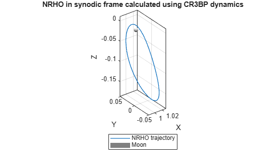
This section plots the orbit found in the synodic frame of reference. The example uses its initial conditions later to construct one in the ephemeris model.
% Compute the trajectory using the initial conditions and time span
% Time span (nondimensional units: one nondimensional time ~ mean motion^-1)
SynodicFrameTimeSpan = linspace(0, targetPeriod / timeScaleFactor, timePoints);
synodicFrameIntegrationOptions = odeset('RelTol', 1e-10, 'AbsTol', 1e-10);

% use ode45 to integrate the initial conditions over one period
[~, synodicFrameNRHOState] = ...
    ode45(@(t, synodicFrameNRHOState) ...
    CR3BPDynamics(synodicFrameNRHOState, mu), ...
    SynodicFrameTimeSpan, ...
    initialStateCR3BP, ...
    synodicFrameIntegrationOptions);

plot3(synodicFrameNRHOState(:, 1), synodicFrameNRHOState(:, 2), synodicFrameNRHOState(:, 3), LineWidth=1)
hold on

[X,Y,Z] = sphere(250);
surf(X * moonRadius / lengthScaleFactor + (1 - mu), ...
Y * moonRadius / lengthScaleFactor, ...
Z * moonRadius / lengthScaleFactor, ...
EdgeColor="none");

xlabel("X");
ylabel("Y");
zlabel("Z");
title("NRHO in synodic frame calculated using CR3BP dynamics");
legend("NRHO trajectory", "Moon", Location = 'southoutside');
axis equal
grid on
box on
colormap gray
Ephemeris Model Initial State
In this section calculateEphemerisRestrictedStates refines the node states by enforcing consistency when the solver propagates them with the point-mass Earth gravity and ephemeris-based Moon perturbations. The function finally converts the first node into a dimensional Moon-centered inertial position and velocity, rotates it out of the synodic frame, and translates it by the Moon state, yielding the initial conditions used for the long ephemeris propagation.
if recalculateOrbit
    numericalOptions = Aero.spacecraft.NumericalPropagatorOptions(GravitationalPotentialModel = "point-mass"); %#ok<UNRCH>
    thirdBodyOptions(numericalOptions, IncludeThirdBodyGravity = true, ThirdBodyGravitySource = "Moon");

    % Initial state in ephemeris model
    nodeStatesEphemeris = calculateEphemerisRestrictedStates(nodeStates, ...
        nodeTimes, ...
        numStates, ...
        numNodes, ...
        numericalOptions, ...
        lengthScaleFactor, ...
        timeScaleFactor, ...
        icrfToSynodicTransformAtNodes, ...
        moonPositionAtNodes, ...
        moonVelocityAtNodes, ...
        startTime);

    % Dimensional initial state (Moon-centered, inertial)
    initialPosition = nodeStatesEphemeris(1:3, 1) * lengthScaleFactor * 1e3;
    initialVelocity = nodeStatesEphemeris(4:6, 1) * (lengthScaleFactor / timeScaleFactor) * 1e3;

    initialPosition = icrfToSynodicTransformAtNodes(:, :, 1)' * initialPosition;
    initialVelocity = icrfToSynodicTransformAtNodes(:, :, 1)' * initialVelocity;

    initialPosition = moonPositionAtNodes(:, 1) + initialPosition;
    initialVelocity = moonVelocityAtNodes(:, 1) + initialVelocity;

    % Save the relevant variables
    save("NRHOdata.mat", ...
        "initialStateCR3BP", ...
        "initialPosition", ...
        "initialVelocity");
end
Ephemeris Model Orbit Propagation Using Satellite Scenario
This section propagates the orbit in the Earth-centered inertial frame with point-mass gravitational potential model for Earth and Moon using satelliteScenario. A physical time vector from startTime to endTime is built with uniform sampling, and the spacecraft state is integrated over time. These baseline states underpin all later visualizations and also serve as reference trajectories for navigation and guidance algorithm development or link-budget and coverage analysis.
% Time vector for the NRHO trajectory
endTime   = startTime + seconds(numOrbits * targetPeriod);
timeVector = linspace(startTime, endTime, timePoints);
sampleTime = seconds(timeVector(2) - timeVector(1));

% Create scenario spanning the propagated interval
scenario = satelliteScenario(startTime, endTime, sampleTime);
numericalPropagator(scenario, ...
    GravitationalPotentialModel="point-mass", ...
    IncludeThirdBodyGravity=true, ...
    ThirdBodyGravitySource="Moon");

% Satellite
[a,ecc,incl,RAAN,argp,nu] = ijk2keplerian(initialPosition, initialVelocity);
nrhoSpacecraft = satellite(scenario, a,ecc,incl,RAAN,argp,nu, Name="NRHO Spacecraft", OrbitPropagator="numerical");

% Retrieve the ICRF position vector of the satellite.
positionsInertial = states(nrhoSpacecraft);
positionsInertial = positionsInertial';
Visualization in Moon-Centered Frame
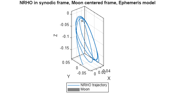
This section turns the raw trajectory data into plots you can inspect directly. This plot shows the NRHO in the synodic frame in a Moon-centered frame of reference. Seeing the orbit helps link the mathematical construction in the CR3BP to the operational picture relevant for communications, access to the lunar surface, and long-term mission planning.
% Moon position at each time step
[~, moonOrbitInertial] = ...
    moonDataAtNodes(length(timeVector), timeVector, 1, timeVector(1));
moonOrbitInertial = moonOrbitInertial';

% Convert ICRF position of the satellite to synodic frame
positionsSynodic = convertOrbitInCR3BP(positionsInertial, moonOrbitInertial, mu, lengthScaleFactor);
positionSynodicRelativeToMoon = positionsSynodic - [1 - mu, 0, 0];

% NRHO in synodic frame (3D)
figure(Name="NRHO in synodic frame, Moon centered", Color="w");
plot3(positionSynodicRelativeToMoon(:, 1), ...
positionSynodicRelativeToMoon(:, 2), ...
positionSynodicRelativeToMoon(:, 3), ...
LineWidth=1);
hold on
[X,Y,Z] = sphere(250);
surf(X * moonRadius / lengthScaleFactor, ...
Y * moonRadius / lengthScaleFactor, ...
Z * moonRadius / lengthScaleFactor, ...
EdgeColor="none");
xlabel("X");
ylabel("Y");
zlabel("Z");
title("NRHO in synodic frame, Moon centered frame, Ephemeris model");
legend("NRHO trajectory", "Moon", Location = 'southoutside');
colormap gray
axis equal
grid on
box on
Satellite Scenario Visualization
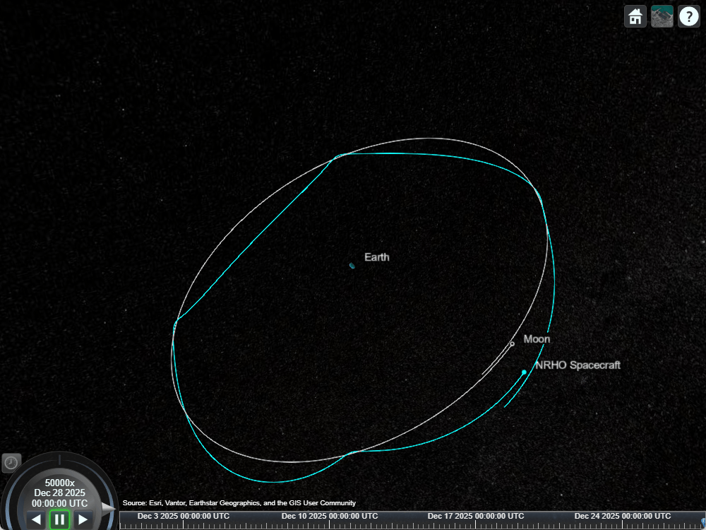
This section loads the calculated trajectory into Satellite Scenario to visualize the NRHO in ICRF interactively. An "Earth" ground station serves as a visual label at the planet. By using satelliteScenarioViewer and play(scenario), you can animate the motion, change camera viewpoints, and overlay additional assets such as real ground sites or prospective lunar surface stations.
% Add ground station to label Earth (latitude and longitude in degrees)
earth = groundStation(scenario, 90, 0, Name="Earth");
earth.MarkerSize = 0.001;

% Set the satellite lead time to 0 and trail time to span the scenario
% duration
nrhoSpacecraft.Orbit.LeadTime = 0;
nrhoSpacecraft.Orbit.TrailTime = seconds(scenario.StopTime - scenario.StartTime);

% Create a viewer with useful overlays
viewer = satelliteScenarioViewer(scenario, ...
    ShowDetails=true, ...
    CameraReferenceFrame="Inertial", ...
    PlaybackSpeedMultiplier=50000);

% Show the orbit of the Moon, set the lead time to 0, trail time to span
% the scenario duration and marker size to 6
moon = centralBodyOptions(scenario, CentralBody="Moon");
moon.MarkerSize = 6;
show(moon.Orbit);
moon.Orbit.LeadTime = 0;
moon.Orbit.TrailTime = seconds(scenario.StopTime - scenario.StartTime);

% Adjust the camera position
campos(viewer, ...
    30, ...                          % Latitude, deg
    -100, ...                        % Longitude, deg
    lengthScaleFactor * 1e3 * 3);    % Altitude, m

% Play the scenario
play(scenario);
Function Definitions
This section implements the dynamics and constraints that connect the CR3BP-based NRHO design to the ephemeris-based refinement. Helper utilities such as radii and CR3BPDynamics define the normalized three-body environment and geometry. Helper utilities such as radii and CR3BPDynamics define the normalized three-body environment and geometry. The multiple-shooting tools (calculateCR3BPstates, calculateResidualForCR3BPMultipleShooting, unpackStates) solve for a periodic orbit in the synodic frame. The ephemeris tools (calculateEphemerisRestrictedStates, calculateResidualForEphemerisRestrictedMultipleShooting, costEphemeris) enforce stitching and closure when the nodes are propagated with propagateOrbit in a realistic Earth–Moon model. Finally, moonDataAtNodes builds the bridge between these worlds by querying DE405 ephemeris and constructing a Moon-centered synodic frame at each node.
The radii function calculates the 3D distance of the spacecraft from the primaries.
function [rPrimary, rSecondary] = radii(state, mu)
    x = state(1);
    y = state(2);
    z = state(3);

    rPrimary   = sqrt((x + mu)^2       + y^2 + z^2);
    rSecondary = sqrt((x - 1 + mu)^2   + y^2 + z^2);
end
The CR3BPDynamics function encodes the normalized CR3BP equations of motion in the synodic Earth–Moon frame. It combines gravitational accelerations from the two primaries with the Coriolis and centrifugal terms that arise in the synodic frame. By packaging the dynamics in this way, the same model can be used seamlessly for both forward propagation (through ode45) and in the multiple-shooting residual calculations, ensuring that the NRHO design and verification are based on a consistent physical model.
function dStateDt = CR3BPDynamics(state, mu)
    x  = state(1);
    y  = state(2);
    z  = state(3);
    vx = state(4);
    vy = state(5);
    vz = state(6);

    % Calculate the radii
    [rPrimary, rSecondary] = radii([x; y; z], mu);

    % CR3BP state derivatives
    ax = 2 * vy + x - (1 - mu) * (x + mu) / rPrimary^3 - mu * (x - 1 + mu) / rSecondary^3;
    ay = -2 * vx + y - (1 - mu) * y / rPrimary^3 - mu * y / rSecondary^3;
    az = -(1 - mu) * z / rPrimary^3 - mu * z / rSecondary^3;

    % Assemble the derivative of the state with respect to time
    dStateDt = [vx; vy; vz; ax; ay; az];
end
The calculateCR3BPstates function builds the NRHO using CR3BP dynamics. The NRHO is calculated using multiple shooting, where the trajectory representing one period is broken into segments representing smaller time intervals. In each segment, an initial value problem is solved with its own guessed initial conditions. The segment solutions are then stitched together by enforcing continuity at segment transitions and, because the NRHO is a periodic orbit, the states at the beginning of the first segment must equal the states at the end of the last segment. Additionally, the formulation enforces symmetry with respect to the XZ plane by imposing the initial, and so the last, Y component of the spacecraft position to be zero.
function [nodeStates, nodeTimes] = calculateCR3BPstates(mu, numStates, numNodes, targetPeriod) %#ok<DEFNU>
    % Multiple-shooting initial guess for the state
    % of the spacecraft to produce an NRHO.
    x0  = 1.021;
    y0  = 0;
    z0  = -0.18;
    vx0 = 0;
    vy0 = -0.101;
    vz0 = 0;

    initialStateGuess = [x0; y0; z0; vx0; vy0; vz0];

    % Node times over one period
    nodeTimes = linspace(0, targetPeriod, numNodes);

    % Propagate initial guess to obtain state values at each node
    [~, stateSamples] = ode45(@(t, state) CR3BPDynamics(state, mu), ...
        nodeTimes, ...
        initialStateGuess, ...
        odeset(RelTol=1e-10, AbsTol=1e-10));

    stateSamples = stateSamples.';
    stateVectorGuess = stateSamples(:);

    % Configure options for fsolve
    solverOptions = optimoptions( ...
        @fsolve, ...
        Display                = "iter", ...
        MaxFunctionEvaluations = 1e6, ...
        StepTolerance          = 1e-9, ...
        FunctionTolerance      = 1e-9, ...
        MaxIterations          = 1e3, ...
        Algorithm              = 'levenberg-marquardt');

    % Solve for consistent node states
    disp("Calculating NRHO initial conditions.");
    stateVectorSolution = fsolve(@(stateVector) calculateResidualForCR3BPMultipleShooting(stateVector, ...
        mu, ...
        numNodes, ...
        numStates, ...
        targetPeriod, ...
        odeset(RelTol=1e-6, AbsTol=1e-6)), ...
        stateVectorGuess, ...
        solverOptions);

    % Convert 1-D state vector to numStates-by-numNodes matrix
    nodeStates = unpackStates(stateVectorSolution, numNodes, numStates);
end
The calculateResidualForCR3BPMultipleShooting function constructs the nonlinear system that fsolve drives to zero in the CR3BP multiple-shooting problem. It unpacks the node states, propagates each node forward to the next using CR3BPDynamics, and builds residuals that measure the mismatch between propagated and stored end states. Additional residuals enforce full-period closure (start and end nodes match) and a symmetry constraint so that the initial state lies on the XZ plane (Y coordinate is 0). When these residuals are near zero, the node states describe a smoothly stitched, periodic NRHO in the synodic frame.
function residual = calculateResidualForCR3BPMultipleShooting(stateVector, mu, numNodes, numStates, targetPeriod, odeOptions)
    % Packs multiple-shooting states and enforces stitching and closure.
    nodeStates = unpackStates(stateVector, numNodes, numStates);

    % Node times over the full period
    nodeTimes = linspace(0, targetPeriod, numNodes);

    % Dynamic stitching of residuals (propagate node k -> k+1)
    dynamicResidual = zeros(numStates * (numNodes - 1), 1);
    for k = 1:(numNodes - 1)
        stateK   = nodeStates(:, k);
        timeK    = nodeTimes(k);
        timeKp1  = nodeTimes(k + 1);

        [~, localState] = ode45(@(t, state) CR3BPDynamics(state, mu), [timeK, timeKp1], stateK, odeOptions);

        dynamicResidual(((k - 1) * numStates + 1):(k * numStates)) = localState(end, :).'-nodeStates(:, k + 1);
    end

    % Full-period closure and constraint y(0) = 0
    closureResidual = nodeStates(:, end) - nodeStates(:, 1);

    residual = [dynamicResidual; closureResidual; nodeStates(2, 1)];
end
The calculateEphemerisRestrictedStates function upgrades the CR3BP multiple-shooting solution into a high-fidelity ephemeris-based NRHO by using the CR3BP solution as the initial guess to construct the ephemeris model NRHO. It treats all node states as a decision vector and uses fmincon to minimize costEphemeris subject to the stitching and closure constraints from calculateResidualForEphemerisRestrictedMultipleShooting. Internally, these constraints propagate each node forward in an Earth-centered inertial frame using propagateOrbit and compare the propagated state with the next node. In an ephemeris restricted model, the solver cannot achieve a truly periodic orbit but only a quasi-periodic one. The formulation enforces periodicity by minimizing the state deviation after one period with respect to the initial value.
function nodeStatesEphemeris = calculateEphemerisRestrictedStates(nodeStates, ...
    nodeTimes, ...
    numStates, ...
    numNodes, ...
    numericalOptions, ...
    lengthScaleFactor, ...
    timeScaleFactor, ...
    icrfToSynodicTransformAtNodes, ...
    moonPositionAtNodes, ...
    moonVelocityAtNodes, ...
    startTime) %#ok<DEFNU>

    % Decision vector
    stateVectorGuess = nodeStates(:);

    % Configure options for fmincon
    optimizerOptions = optimoptions( ...
        @fmincon, ...
        Display                = "iter", ...
        MaxFunctionEvaluations = 1e6, ...
        StepTolerance          = 1e-9, ...
        FunctionTolerance      = 1e-9, ...
        ConstraintTolerance    = 1e-7, ...
        MaxIterations          = 1e5);

    % Solve for node states in the ephemeris model
    disp("Calculating NRHO in ephemeris model.");
    stateVectorSolution = fmincon(@(stateVector)  costEphemeris(stateVector, ...
        numStates, ...
        numNodes, ...
        lengthScaleFactor, ...
        timeScaleFactor, ...
        icrfToSynodicTransformAtNodes, ...
        moonPositionAtNodes, ...
        moonVelocityAtNodes), ...
        stateVectorGuess, ...
        [], [], [], [], [], [], ...
        @(stateVector) calculateResidualForEphemerisRestrictedMultipleShooting(...
        stateVector, ...
        nodeTimes, ...
        numStates, ...
        numNodes, ...
        numericalOptions, ...
        lengthScaleFactor, ...
        timeScaleFactor, ...
        icrfToSynodicTransformAtNodes, ...
        moonPositionAtNodes, ...
        moonVelocityAtNodes, ...
        startTime), ...
        optimizerOptions);

    % Extract states
    nodeStatesEphemeris = unpackStates(stateVectorSolution, numNodes, numStates);
end
The calculateResidualForEphemerisRestrictedMultipleShooting function builds the nonlinear equality constraints that enforce consistency of the node states in the ephemeris model. It converts the CR3BP-scaled node states into dimensional inertial position and velocity, adds the Moon's inertial state to convert the state into the Earth-centered reference frame, and then propagates each node forward to the next using propagateOrbit. The differences between propagated and stored node states form dynamic stitching residuals. Additional residuals enforce that the orbit starts and ends at symmetric locations in a Moon-centered frame. When these residuals are near zero, the node states describe a smoothly stitched, nearly periodic NRHO in the realistic Earth–Moon environment.
function [cInequality, equalityResidual] = calculateResidualForEphemerisRestrictedMultipleShooting(stateVector, ...
    nodeTimes, ...
    numStates, ...
    numNodes, ...
    numericalOptions, ...
    lengthScaleFactor, ...
    timeScaleFactor, ...
    icrfToSynodicTransformAtNodes, ...
    moonPositionAtNodes, ...
    moonVelocityAtNodes, ...
    startTime)

    nodeStates = unpackStates(stateVector, numNodes, numStates);

    positionNodes = zeros(3, numNodes);
    velocityNodes = zeros(3, numNodes);

    % Dimensional times, with scaled period
    timeDimensional = nodeTimes * timeScaleFactor;

    for k = 1:numNodes
        % since icrfToSynodicTransformAtNodes is orthonormal, its transpose
        % gives the inverse transform
        positionNodes(:, k) = nodeStates(1:3, k) * lengthScaleFactor * 1e3;
        positionNodes(:, k) = icrfToSynodicTransformAtNodes(:, :, k)' * positionNodes(:, k);

        velocityNodes(:, k) = nodeStates(4:6, k) * (lengthScaleFactor / timeScaleFactor) * 1e3;
        velocityNodes(:, k) = icrfToSynodicTransformAtNodes(:, :, k)' * velocityNodes(:, k);

        positionNodes(:, k) = moonPositionAtNodes(:, k) + positionNodes(:, k);
        velocityNodes(:, k) = moonVelocityAtNodes(:, k) + velocityNodes(:, k);
    end

    % Dynamic stitching of residuals (propagate node k -> k+1)
    dynamicResidual = zeros(numStates * (numNodes - 1), 1);
    for k = 1:(numNodes - 1)
        positionK = positionNodes(:, k);
        velocityK = velocityNodes(:, k);

        timeK   = startTime + seconds(timeDimensional(k));
        timeKp1 = startTime + seconds(timeDimensional(k + 1));

        [positionKp1, velocityKp1] = propagateOrbit( ...
            timeKp1, ...
            positionK, velocityK, ...
            Epoch                   = timeK, ...
            PropModel               = "numerical", ...
            NumericalPropagatorOptions = numericalOptions, ...
            InputCoordinateFrame    = "inertial", ...
            OutputCoordinateFrame   = "inertial");

        % final dynamic residuals
        dynamicResidual(((k - 1) * numStates + 1):(k * numStates)) = ...
            [ (positionKp1 - positionNodes(:, k + 1)) / (lengthScaleFactor * 1e3); ...
              (velocityKp1 - velocityNodes(:, k + 1)) / ((lengthScaleFactor / timeScaleFactor) * 1e3) ];
    end

    % spacecraft position with respect to the Moon
    positionStartMoon = icrfToSynodicTransformAtNodes(:, :, 1) * (positionNodes(:, 1)...
        - moonPositionAtNodes(:, 1)) / (lengthScaleFactor * 1e3);
    positionEndMoon = icrfToSynodicTransformAtNodes(:, :, end) * (positionNodes(:, end)...
        - moonPositionAtNodes(:, end)) / (lengthScaleFactor * 1e3);

    % equality residuals
    equalityResidual = [dynamicResidual; positionStartMoon(2); positionEndMoon(2)];
    cInequality      = [];
end
The costEphemeris function defines the scalar objective minimized during ephemeris refinement. After mapping the node states into dimensional Moon-centered coordinates, it measures how well the start and end of the orbit match in both position and velocity. Squared norms of these mismatches form the cost, so minimizing the cost drives the solution toward a closed, symmetric NRHO in the ephemeris model. By combining this cost with the dynamic stitching constraints, the optimization problem promotes global periodicity of the orbit.
function costValue = costEphemeris(stateVector, ...
    numStates, ...
    numNodes, ...
    lengthScaleFactor, ...
    timeScaleFactor, ...
    icrfToSynodicTransformAtNodes, ...
    moonPositionAtNodes, ...
    moonVelocityAtNodes)

    nodeStates = unpackStates(stateVector, numNodes, numStates);

    % Initialize vectors
    positionNodes = zeros(3, 2);
    velocityNodes = zeros(3, 2);

    % Calculate state at the first node
    positionNodes(:, 1) = nodeStates(1:3, 1) * lengthScaleFactor * 1e3;
    positionNodes(:, 1) = icrfToSynodicTransformAtNodes(:, :, 1)' * positionNodes(:, 1);

    velocityNodes(:, 1) = nodeStates(4:6, 1) * (lengthScaleFactor / timeScaleFactor) * 1e3;
    velocityNodes(:, 1) = icrfToSynodicTransformAtNodes(:, :, 1)' * velocityNodes(:, 1);

    positionNodes(:, 1) = moonPositionAtNodes(:, 1) + positionNodes(:, 1);
    velocityNodes(:, 1) = moonVelocityAtNodes(:, 1) + velocityNodes(:, 1);

    % Calculate state at the last node
    positionNodes(:, end) = nodeStates(1:3, end) * lengthScaleFactor * 1e3;
    positionNodes(:, end) = icrfToSynodicTransformAtNodes(:, :, end)' * positionNodes(:, end);

    velocityNodes(:, end) = nodeStates(4:6, end) * (lengthScaleFactor / timeScaleFactor) * 1e3;
    velocityNodes(:, end) = icrfToSynodicTransformAtNodes(:, :, end)' * velocityNodes(:, end);

    positionNodes(:, end) = moonPositionAtNodes(:, end) + positionNodes(:, end);
    velocityNodes(:, end) = moonVelocityAtNodes(:, end) + velocityNodes(:, end);

    % Calculate the state with respect to the Moon
    positionStartMoon = icrfToSynodicTransformAtNodes(:, :, 1) * (positionNodes(:, 1)...
        - moonPositionAtNodes(:, 1)) / (lengthScaleFactor * 1e3);
    velocityStartMoon = icrfToSynodicTransformAtNodes(:, :, 1) * (velocityNodes(:, 1)...
        - moonVelocityAtNodes(:, 1)) / ((lengthScaleFactor / timeScaleFactor) * 1e3);

    positionEndMoon = icrfToSynodicTransformAtNodes(:, :, end) * (positionNodes(:, end)...
        - moonPositionAtNodes(:, end)) / (lengthScaleFactor * 1e3);
    velocityEndMoon = icrfToSynodicTransformAtNodes(:, :, end) * (velocityNodes(:, end)...
        - moonVelocityAtNodes(:, end)) / ((lengthScaleFactor / timeScaleFactor) * 1e3);

    % Calculate the error and the cost value
    positionError = positionEndMoon - positionStartMoon;
    velocityError = velocityEndMoon - velocityStartMoon;

    costValue = norm(positionError)^2 + norm(velocityError)^2;
end
The moonDataAtNodes function queries the DE405 ephemeris at each node time to obtain the Moon's Earth-centered inertial position and velocity, then constructs a local synodic frame aligned with the Moon's motion. The X axis points from Earth to the Moon, the Z axis aligns with the normal direction to the Moon's orbital plane, and the Y axis completes the right-hand rule. This co-rotating frame provides a natural bridge between CR3BP-scaled states and dimensional inertial states, and it is used to express closure constraints and mapping operations in a Moon-centered perspective that closely matches how the NRHO would be flown in practice.
function [icrfToSynodicTransformAtNodes, moonPositionAtNodes, moonVelocityAtNodes] = ...
    moonDataAtNodes(numNodes, ...
    nodeTimes, ...
    timeScaleFactor, ...
    startTime)

    % Moon position and velocity at the nodes (Earth-centered inertial).
    icrfToSynodicTransformAtNodes = zeros(3, 3, numNodes);
    moonPositionAtNodes    = zeros(3, numNodes);
    moonVelocityAtNodes    = zeros(3, numNodes);

    for idx = 1:numNodes
        if ~isdatetime(nodeTimes)
            dateTimeCurrent = startTime + seconds(nodeTimes(idx) * timeScaleFactor);
        else
            dateTimeCurrent = nodeTimes(idx);
        end

        % Correct for Julian time
        taiMinusUtc = 37;
        ttMinusTai  = 32.184;
        dateTimeTt  = dateTimeCurrent + seconds(taiMinusUtc) + seconds(ttMinusTai);
        timeJulian  = tdbjuliandate([ ...
            dateTimeTt.Year, ...
            dateTimeTt.Month, ...
            dateTimeTt.Day, ...
            dateTimeTt.Hour, ...
            dateTimeTt.Minute, ...
            dateTimeTt.Second]);

        % Retrieve the position and velocity of the Moon
        [moonPositionCurrent, moonVelocityCurrent] = planetEphemeris(timeJulian, "Earth", "Moon", "405");

        moonPositionCurrent = moonPositionCurrent.' * 1e3;
        moonVelocityCurrent = moonVelocityCurrent.' * 1e3;

        % Build the icrfToSynodicTransformAtNodes matrix, for each node
        xAxis = moonPositionCurrent / norm(moonPositionCurrent);
        yAxis = moonVelocityCurrent / norm(moonVelocityCurrent);
        zAxis = cross(xAxis, yAxis);
        zAxis = zAxis / norm(zAxis);
        yAxis = cross(zAxis, xAxis);

        icrfToSynodicTransformAtNodes(:, :, idx) = [xAxis yAxis zAxis].';

        moonPositionAtNodes(:, idx) = moonPositionCurrent;
        moonVelocityAtNodes(:, idx) = moonVelocityCurrent;
    end
end
The unpackStates utility reshapes the flat decision vector used by the solvers into a numStates-by-numNodes matrix of node states. Keeping this logic in a dedicated function makes the multiple-shooting code more readable and reduces the chance of indexing errors if you add or remove states or nodes from the formulation.
function nodeStates = unpackStates(stateVector, numNodes, numStates)
    % Unpack decision vector into node states
    numVariables = numStates * numNodes;
    nodeStates   = reshape(stateVector(1:numVariables), [numStates, numNodes]);
end
The convertOrbitInCR3BP function transforms the propagated inertial orbit back to the nondimensional synodic frame to later plot it.
function positionsSynodic = convertOrbitInCR3BP(positionsInertial, moonOrbitInertial, mu, lengthScaleFactor)
    numPoints = size(positionsInertial, 1);

    vMoon = [zeros(1, 3); diff(moonOrbitInertial)];

    % Build the icrfToSynodicTransformAtNodes matrix, for each point in the orbit
    icrfToSynodicTransformAtNodes = zeros(3, 3, numPoints);
    for idx = 1:numPoints
        xAxis = moonOrbitInertial(idx, :).';
        xAxis = xAxis / norm(xAxis);

        vDir = vMoon(idx, :).';
        if norm(vDir) < eps && idx < numPoints
            vDir = (moonOrbitInertial(idx + 1, :) - moonOrbitInertial(idx, :)).';
        elseif norm(vDir) < eps && idx > 1
            vDir = (moonOrbitInertial(idx, :) - moonOrbitInertial(idx - 1, :)).';
        end
        vDir = vDir / norm(vDir);

        zAxis = cross(xAxis, vDir);
        zAxis = zAxis / norm(zAxis);
        yAxis = cross(zAxis, xAxis);

        icrfToSynodicTransformAtNodes(:, :, idx) = [xAxis yAxis zAxis].';
    end

    % Use the icrfToSynodicTransformAtNodes matrix to transform each point in the orbit
    rMoonRelative = positionsInertial - moonOrbitInertial;
    positionsSynodic = zeros(numPoints, 3);
    for idx = 1:numPoints
        rotated = icrfToSynodicTransformAtNodes(:, :, idx) * rMoonRelative(idx, :).';
        positionsSynodic(idx, :) = rotated.' / (lengthScaleFactor * 1e3) + [1 - mu, 0, 0];
    end
end
References
[1] Bucci, L., Colagrossi, A., & Lavagna, M. (2018). Rendezvous in Lunar near rectilinear halo orbits. Advances in Astronautics Science and Technology, 1(1), 39–43.
[2] E. Zimovan, K. Howell, and D. Davis, “Near Rectilinear Halo Orbits and Their Application in Cis-Lunar Space,” 3rd IAA Conference on Dynamics and Control of Space Systems, May 2017.
[3] NASA NSSDC Planetary Data: https://nssdc.gsfc.nasa.gov/planetary/factsheet/moon.
[4] National Geospatial-Intelligence Agency. "World Geodetic System 1984: Its Definition and Relationships with Local Geodetic Systems." Version 1.0.0, Department of Defense, 8 July 2014.
See Also
eclipse | access | groundStation

