propagateOrbit
Syntax
Description
[
calculates the positions and velocities in the International Celestial Reference Frame
(ICRF) corresponding to the time specified by positions
,velocities
] = propagateOrbit(time
,gpStruct
)time
using the
two-line-element (TLE) or orbit mean-elements message (OMM) data.
[
calculates the positions and velocities using specified orbital elements to define epoch
states. The function assumes that the epoch is the first element in the
positions
,velocities
] = propagateOrbit(time
,a
,ecc
,incl
,RAAN
,argp
,nu
)time
argument.
[
calculates the positions and velocities at the epoch defined by positions
,velocities
] = propagateOrbit(time
,rEpoch
,vEpoch
)rEpoch
and vEpoch
. The function assumes that the epoch is the first element in
the time
argument.
[
calculates the positions and velocities using additional parameters specified by one or more
name-value arguments.positions
,velocities
] = propagateOrbit(___,Name=Value
)
Examples
Read the data from the TLE (Two-Line Element) file named 'leoSatelliteConstellation.tle
'. Calculate the position and velocity based on the TLE structure, 'tleStruct'
. This file is located on the MATLAB® path and is provided with the Aerospace Toolbox.
tleStruct = tleread('leoSatelliteConstellation.tle')
tleStruct=40×1 struct array with fields:
Name
SatelliteCatalogNumber
Epoch
BStar
RightAscensionOfAscendingNode
Eccentricity
Inclination
ArgumentOfPeriapsis
MeanAnomaly
MeanMotion
Calculate the position and velocity corresponding to the input time using the TLE data defined in tleStruct
.
[r,v] = propagateOrbit(datetime(2022, 1, 3, 12, 0, 0),tleStruct);
This examples shows how to simulate a lunar free-return trajectory using numerical propagator. Define trajectory start and end times.
startTime = datetime(2022,11,17,14,40,0); endTime = datetime(2022,11,24,12,45,0);
Construct datetime vector representing the trajectory time stamps spaced at 60 second intervals.
sampleTime = 60; % s
time = startTime:seconds(sampleTime):endTime;
Define the initial position and velocity of the spacecraft in ICRF. These represent the spacecraft states immediately after the translunar injection burn.
initialPosition = [5927630.386747557; ... 3087663.891097251; ... 1174446.969646237]; initialVelocity = [-5190.330300215130; ... 8212.486957313564; ... 4605.538019512981];
Define the options for numerical orbit propagation. Configure the ordinary differential equation (ODE) solver options, gravitational potential model and the third body gravity. Include third body gravity from all supported solar system bodies. Note that the numerical propagator also supports inclusion of perturbations due to drag from Earth atmosphere and solar radiation pressure. However, these effects are ignored in this example.
numericalPropOpts = Aero.spacecraft.NumericalPropagatorOptions( ... ODESet=odeset(RelTol=1e-8,AbsTol=1e-8,MaxStep=300), ... IncludeThirdBodyGravity=true, ... ThirdBodyGravitySource=[ ... "Sun" ... "Mercury" ... "Venus" ... "Moon" ... "Mars" ... "Jupiter" ... "Saturn" ... "Uranus" ... "Neptune" ... "Pluto"], ... GravitationalPotentialModel="point-mass")
numericalPropOpts = NumericalPropagatorOptions with properties: ODESolver: "ode45" ODESet: [1×1 struct] CentralBodyOptions: [1×1 Aero.spacecraft.CentralBodyOptions] GravitationalPotentialModel: "point-mass" IncludeAtmosDrag: 0 IncludeThirdBodyGravity: 1 ThirdBodyGravitySource: ["Sun" "Mercury" "Venus" "Moon" "Mars" "Jupiter" "Saturn" "Uranus" "Neptune" "Pluto"] IncludeSRP: 0 PlanetaryEphemerisModel: "de405"
Define the physical properties (mass, reflectivity coefficient and solar radiation pressure area) of the spacecraft.
physicalProps = Aero.spacecraft.PhysicalProperties( ... Mass=10000, ... ReflectivityCoefficient=0.3, ... SRPArea=2)
physicalProps = PhysicalProperties with properties: Mass: 10000 DragCoefficient: 2.1790 DragArea: 1 ReflectivityCoefficient: 0.3000 SRPArea: 2
Propagate the spacecraft trajectory. While PropModle name-value argument defaults to "numerical" if you explicitly specify NumericalPropagatorOptions or PhysicalProperties name-value argument, PropModel has been explicitly specified for illustrative purposes.
position = propagateOrbit( ... time, ... initialPosition, ... initialVelocity, ... PropModel="numerical", ... NumericalPropagatorOptions=numericalPropOpts, ... PhysicalProperties=physicalProps);
Convert the position history to timetable.
positionTT = timetable(time',position');
Visualize the trajectory on a satellite scenario viewer. To do this, create a satellite scenario object.
sc = satelliteScenario(startTime,endTime,sampleTime);
Add the spacecraft to the scenario using the satellite function and the position timetable.
spacecraft = satellite(sc,positionTT,Name="Spacecraft");
The satellite scenario viewer used for visualizing the scenario already renders visualization for the moon. However, you can gain better situational awareness if the lunar orbit is plotted as well. To do this, add a satellite to the scenario using the satellite function that is on the same trajectory as that of the Moon. To calculate the trajectory of the Moon, start by computing the barycentric dynamical times (TDB) for the simulation time samples as Julian dates.
leapSeconds = 37; ttMinusTAI = 32.184; terrestrialTime = time + seconds(leapSeconds + ttMinusTAI); tdbJD = tdbjuliandate([ ... terrestrialTime.Year' ... terrestrialTime.Month' ... terrestrialTime.Day' ... terrestrialTime.Hour' ... terrestrialTime.Minute' ... terrestrialTime.Second']);
Calculate the positions of the Moon for each scenario time sample using planetEphemeris and convert the positions into a timetable.
pMoonkm = planetEphemeris(tdbJD,"earth","moon"); % km pMoon = convlength(pMoonkm,'km','m'); % m pMoonTT = timetable(time',pMoon);
Add a satellite representing the Moon to the scenario using the satellite function. Set the orbit and marker color to red.
moon = satellite(sc,pMoonTT,Name="Moon"); moon.Orbit.LineColor="red"; moon.MarkerColor="red";
The scale of the distance involved in the scenario is large enough that the Earth may not be readily visible when viewing from the shadow side. To mitigate this, add a ground station at the North pole of the Earth and label it "Earth". Set the marker size of this ground station to 0.001. This way, the label "Earth" will always be visible near the position of the Earth.
earth = groundStation(sc, ... 90, ... % Latitude, deg 0, ... % Longitude, deg Name="Earth"); earth.MarkerSize = 0.001;
Run satelliteScenarioViewer to launch a satellite scenario viewer. Set the playback speed multiplier to 60,000. Set the camera reference frame to "inertial".
v = satelliteScenarioViewer(sc, ... CameraReferenceFrame="Inertial", ... PlaybackSpeedMultiplier=60000);
Set the camera position and orientation to visualize the free-return trajectory from a top-down view.
campos(v, ... 55.991361, ... 18.826434, ... 1163851259.541816); camheading(v, ... 359.7544952991605); campitch(v, ... -89.830968253450209); camroll(v, ... 0);
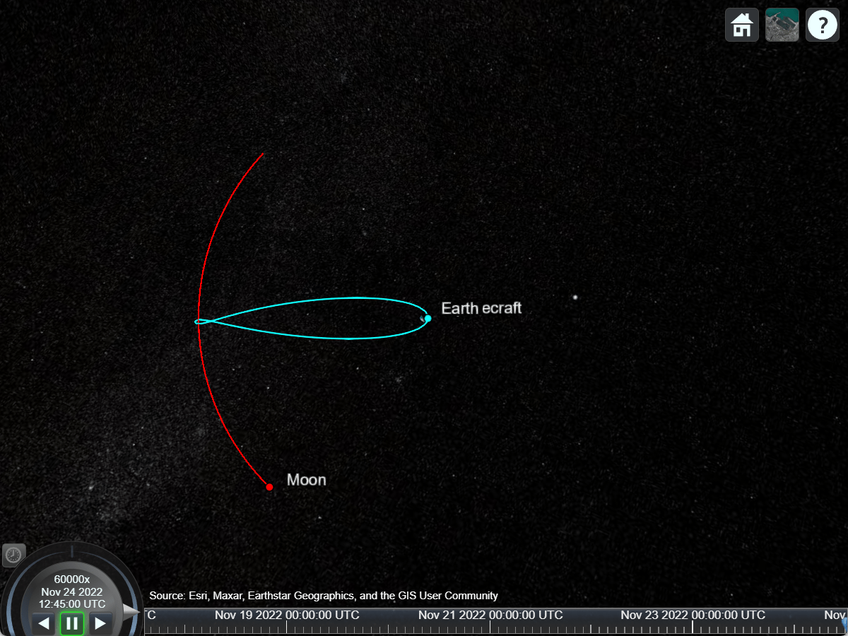
Play the scenario.
play(sc);
Input Arguments
Julian dates or datetime
objects, specified as a
1-by-m vector or m-by-1 vector of doubles or
datetime
objects. time
must be strictly
increasing. This argument represents the times for which the output position and
velocity are reported.
When you specify a datetime
object whose
TimeZone
property is empty, the
propagateOrbit
function assumes that the
datetime
object time zone is UTC.
Example: datetime(2023,6,16)
Example: juliandate(2023,6,16)
Data Types: double
| datetime
Semimajor axes, specified as a numSc-element vector or a scalar,
in meters. If all spacecraft have the same semimajor axis, you can specify
a
as a scalar. numSc is the number of
spacecraft.
Example: 10000000
Example: [8000000 10000000]
Dependencies
If any element of a
is negative, the corresponding element in
ecc
must be greater than or equal to 1. The only supported
PropModel
in this instance is "numerical".
Data Types: double
Orbit eccentricity, which is the deviation of the orbital curve from circular,
specified as a numSc-element vector or scalar. If all spacecraft have
the same eccentricity, you can specify ecc
as a scalar.
numSc is the number of spacecraft.
Example: 0.1
Example: [0.1 0.2]
Dependencies
If any element of ecc
is greater than or equal to 1, the
corresponding element in a
must be negative. The only supported
PropModel
in this instance is
numerical
.
Inclination, which is the vertical tilt of the orbit with respect to the ICRF xy plane measured at the ascending node, specified as a numSc-element vector or a scalar in degrees. numSc is the number of spacecraft.
Example: 10
Example: [20 30]
Right ascension of ascending node (RAAN), specified as a
numSc-element vector or a scalar, in degrees. If all spacecraft have
the same right ascension of ascending node, you can specify RAAN
as
a scalar. numSc is the number of spacecraft.
Example: 10
Example:
[20 30]
Argument of periapsis, which is the angle from the orbit ascending node to periapsis
(closest point of orbit to the central body), specified as a
numSc-element vector or a scalar in degrees. If all spacecraft have
the same argument of periapsis, you can specify RAAN
as a scalar.
numSc is the number of spacecraft.
Example: 10
Example: [20 30]
, if there are two spacecraft
True anomaly, which is the angle between periapsis and the initial position of the
spacecraft, specified as a numSc-element vector or a scalar in
degrees. If all spacecraft have the same true anomaly, you can specify
nu
as a scalar. numSc is the number of
spacecraft.
Example: 10
Example: [20 30]
Position at epoch, specified as a 3-by-1 vector or 3-by-numSc
matrix. If all spacecraft have the same initial position at epoch, you can specify
rEpoch
as a 3-by-1 vector. numSc is the number
of spacecraft. For more information regarding units, see
InputCoordinateFrame
.
Example: [10000000;1000;2000]
Example: [10000000 12000000;1000 2000;2000 4000]
Dependencies
rEpoch
and the corresponding vEpoch
vectors cannot be parallel when PropModel
is set to
'sgp4'
, 'sdp4'
,
'general-perturbations'
or
'two-body-keplerian'
.
Velocity at epoch, specified as a 3-by-1 vector or 3-by-numSc
matrix in m/s. If all spacecraft have the same initial velocity at epoch, you can
specify vEpoch
as a 3-by-1 vector. numSc is the
number of spacecraft.
Example: [0;8000;0]
Example: [0 100;8000 9000;200 300]
Dependencies
vEpoch
and the corresponding rEpoch
vectors cannot be parallel when PropModel
is set to
'sgp4'
, 'sdp4'
,
'general-perturbations'
or
'two-body-keplerian'
.
General perturbations structures representing TLE or OMM data, specified as a
numSc-element vector. numSc is the number of
spacecraft. To create the TLE or OMM data structure, consider using tleread
or
ommread
respectively. For more information on TLE and OMM file structures, see Two Line Element (TLE) Files.
If you specify the CentralBodyOptions
input, set the CentralBody
property of Aero.spacecraft.CentralBodyOptions
to Earth
.
To specify the NumericalPropagatorOptions
input, set the
CentralBody
property of Aero.spacecraft.CentralBodyOptions
to Earth
.
Example: tleread("leoSatelliteConstellation.tle")
Data Types: struct
Name-Value Arguments
Specify optional pairs of arguments as
Name1=Value1,...,NameN=ValueN
, where Name
is
the argument name and Value
is the corresponding value.
Name-value arguments must appear after other arguments, but the order of the
pairs does not matter.
Before R2021a, use commas to separate each name and value, and enclose
Name
in quotes.
Example: PropModel="two-body-keplerian"
specifies
two-body-keplerian
as the propagation method.
Epoch, specified as a scalar datetime
object. The data type of
'Epoch'
is double.
When you specify a datetime
object whose
TimeZone
property is empty, the
propagateOrbit
function assumes that the
datetime
object time zone is UTC.
Example: datetime(2023,6,19)
Default value
Dependencies
When you specify the epoch states using gpStruct
, do not
specify this name-value argument.
Data Types: double
Central body options used for orbit propagation, specified as a Aero.spacecraft.CentralBodyOptions
scalar object. This object specifies the
central body and in the case of the Earth, defines the Earth orientation
parameters.
Default Values
The default value is the object returned by the Aero.spacecraft.CentralBodyOptions
class with the CentralBody property set to Earth
.
Dependencies
You can specify this name-value argument only if PropModel
equals 'two-body-keplerian'
or 'numerical'
.
Additionally, if you set PropModel
to
'numerical'
, the
NumericalPropagatorOptions
argument will be specified by the
central body options already defined by the CentralBodyOptions
property of the Aero.spacecraft.NumericalPropagatorOptions
object specified for the
NumericalPropagatorOptions
argument.
Options used by the numerical orbit propagator, specified as a scalar
Aero.spacecraft.NumericalPropagatorOptions
object.
Default Value
The default value is the object returned when calling the
Aero.spacecraft.NumericalPropagatorOptions
object without any
inputs.
Dependencies
You cannot specify this name-value argument if:
You set
PropModel
to'sgp4'
,'sdp4'
,'general-perturbations'
or'two-body-keplerian'
.You specify the
CentralBodyOptions
name-value argument.
Physical properties of spacecraft used by the numerical orbit propagator,
specified as a scalar or array of
Aero.spacecraft.PhysicalProperties
objects. If all spacecraft use
the same physical properties, you can specify
'PhysicalProperties'
as a scalar.
Default Value
The default value is the object returned when calling the
Aero.spacecraft.PhysicalProperties
object without any
inputs.
Dependencies
If you specify PropModel
to 'sgp4'
,
'sdp4'
, 'general-perturbations'
or
'two-body-keplerian'
, do not specify this name-value
argument.
Orbital state propagation method, specified as one of these values:
"general-perturbations"
—"sgp4"
or"sdp4"
, depending on orbital period. When the orbital period corresponding to the epoch states is less than 225 minutes, the propagation model is"sgp4"
. Otherwise, it is"sdp4"
."two-body-keplerian"
— Two-body Keplerian orbit propagator."sgp4"
— Simplified General Perturbations-4 orbit propagator."sdp4"
— Simplified Deep-Space Perturbations-4 orbit propagator."numerical"
— Numerical propagation model.
Example: PropModel = "two-body-keplerian"
Default Value
"numerical"
— When any one of this is true:You specify epoch states using one of the orbital elements such as
a
,ecc
,incl
,RAAN
,argp
andnu
or position or velocity states such asrEpoch
orvEpoch
and at least one set of states represents a parabolic or hyperbolic orbit. That is, at least one set of orbital elements,a
< 0 andecc
>= 1.Alternatively, at least one set of
rEpoch
andvEpoch
, when converted to inertial frame as rECI and vECI, results in an orbital energy E that is greater than or equal to 0. Assuming mu is the standard gravitational parameter, energy E is calculated asYou explicitly specify
NumericalPropagatorOptions
orPhysicalProperties
name-value arguments.You specify
CentralBodyOptions
name-value argument and theCentralBody
property of the specifiedAero.spacecraft.CentralBodyOptions
class does not equal"Earth"
.
"two-body-keplerian"
— When you specifyCentralBodyOptions
name-value argument and the CentralBody property of the specifiedAero.spacecraft.CentralBodyOptions
class does not equal"Earth"
."general-perturbations"
— For all other cases.
Data Types: char
| string
Aerodynamic drag term, specified as a numSc-element vector or
scalar. If all spacecraft use the same Bstar
value, you can
specify this argument as a scalar. numSc is the number of
spacecraft.
Example: BStar = 0
Example: BStar = [0.0001 0.0002]
, if there are two
spacecraft
Dependencies
propagateOrbit
uses this value when:
Data Types: double
Input coordinate frame of rEpoch
and vEpoch
,
specified as one of these values:
"icrf"
—rEpoch
andvEpoch
are defined in the ICRF in m and m/s, respectively."fixed-frame"
—rEpoch
andvEpoch
are defined as the Earth-centered Earth-fixed (ECEF) frame in m and m/s, respectively."geographic"
—rEpoch
is defined as latitude (deg), longitude (deg), and altitude (m).vEpoch
is defined in the fixed-frame velocity in m/s represented in the north-east-down (NED) frame defined byrEpoch
.
Example: InputCoordinateFrame="fixed-frame"
Data Types: char
| string
Output coordinate frame of output positions
and
velocities
, specified as one of these values:
"icrf"
—positions
andvelocities
are defined in the ICRF in m and m/s respectively."fixed-frame"
—positions
andvelocities
are defined in the Earth-centered Earth-fixed (ECEF) frame in m and m/s respectively."geographic"
—positions
is defined as latitude (deg), longitude (deg), and altitude (m)..velocities
is defined as the fixed-frame velocity in m/s represented in the north-east-down (NED) frame defined by positions.
Example: OutputCoordinateFrame = "geographic"
Data Types: char
| string
Output Arguments
Positions, returned as a 3-by-m-by-numSc array in m/s. m is the number of time samples. numSc is the number of spacecraft.
Velocities, returned as a 3-by-m-by-numSc array in m/s. m is the number of time samples. numSc is the number of spacecraft.
References
[1] Hoots, Felix R., and Ronald L. Roehrich. . Aerospace Defense Command, Peterson AFB CO Office of Astrodynamics, 1980.
[2] Vallado, David, et al. “Revisiting Spacetrack Report #3.” AIAA/AAS Astrodynamics Specialist Conference and Exhibit, American Institute of Aeronautics and Astronautics, 2006. , https://doi.org/10.2514/6.2006-6753.
Version History
Introduced in R2024bYou can now add nonearth central bodies such as Sun
,
Moon
, Mercury
, Venus
,
Mars
, Jupiter
, Saturn
,
Uranus
, and Neptune
. Modify the central body used in
propagateOrbit
using the new Aero.spacecraft.CentralBodyOptions
class and the CentralBodyOptions
input of propagateOrbit
.
The Aerospace Toolbox now incorporates the latest and most accurate equations from https://celestrak.org/publications/AIAA/2006-6753/ in
propagateOrbit
. Both the SGP4 and SDP4 orbit propagators use these
equations and return identical results. The algorithms are detailed in the work of Vallado,
David, et al, “Revisiting Spacetrack Report #3.”, AIAA/AAS
Astrodynamics Specialist Conference and Exhibit, American Institute of
Aeronautics and Astronautics, 2006, https://celestrak.org/publications/AIAA/2006-6753/.
See Also
Objects
Functions
MATLAB Command
You clicked a link that corresponds to this MATLAB command:
Run the command by entering it in the MATLAB Command Window. Web browsers do not support MATLAB commands.
Select a Web Site
Choose a web site to get translated content where available and see local events and offers. Based on your location, we recommend that you select: .
You can also select a web site from the following list
How to Get Best Site Performance
Select the China site (in Chinese or English) for best site performance. Other MathWorks country sites are not optimized for visits from your location.
Americas
- América Latina (Español)
- Canada (English)
- United States (English)
Europe
- Belgium (English)
- Denmark (English)
- Deutschland (Deutsch)
- España (Español)
- Finland (English)
- France (Français)
- Ireland (English)
- Italia (Italiano)
- Luxembourg (English)
- Netherlands (English)
- Norway (English)
- Österreich (Deutsch)
- Portugal (English)
- Sweden (English)
- Switzerland
- United Kingdom (English)