Main Content

pattern

Plot radiation pattern and phase of antenna or array or embedded pattern of antenna element in array

Description

pattern(object,frequency) plots the 3-D radiation pattern of the antenna or array object over a specified frequency. By default, in Antenna Toolbox™, the far-field radius is set to 100λ. For a detailed explanation of field calculation of antennas, see Field Calculation in Antennas.

example

pattern(object,frequency,azimuth,elevation) plots the radiation pattern of the antenna or array object using the specified azimuth and elevation angles.

pattern(___,Name=Value) uses additional options specified by one or more name-value arguments. You can use any of the input arguments from previous syntaxes.

Use the ElementNumber and Termination property to calculate the embedded pattern of the antenna element in an array connected to a voltage source. The voltage source model consists of an ideal voltage source of 1 volt in series with a source impedance. The embedded pattern includes the effect of mutual coupling due to the other antenna elements in the array.

[pat,azimuth,elevation] = pattern(object,frequency,azimuth,elevation) returns the pattern value, pat, value of an antenna or array object at specified frequency. azimuth and elevation are the angles at which the pattern function calculates the directivity.

[pat,azimuth,elevation] = pattern(___,Name=Value) uses additional options specified by one or more name-value arguments.

Examples

collapse all

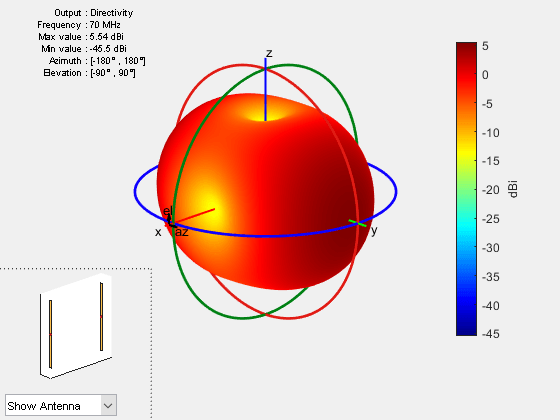
Calculate radiation pattern of default linear array for a frequency of 70 MHZ.

l = linearArray;
pattern(l,70e6)

Figure contains 2 axes objects and other objects of type uicontrol. Axes object 1 contains 6 objects of type patch, surface. Hidden axes object 2 contains 18 objects of type surface, line, text, patch.

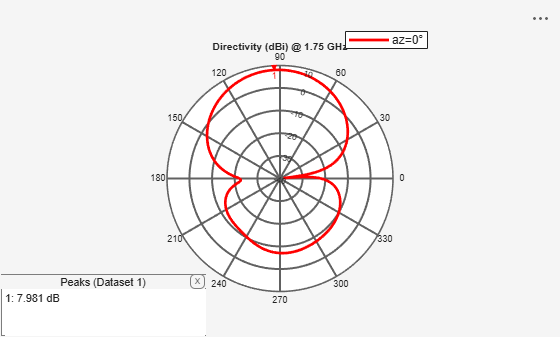
Plot the radiation pattern of a helix antenna in xz-plane.

h = helix; 
pattern (h, 2e9, 0, 1:1:360);

Figure contains an axes object and an object of type uicontainer. The hidden axes object contains 2 objects of type line, text. This object represents az=0° .

[pat,azimuth,elevation] = pattern (h, 2e9, 0, 1:1:360);

Compute the maximum and the minimum value of the radiation pattern and the elevation angle.

pattern_max = max(max(pat))
pattern_max = 
8.7019
pattern_min = min(min(pat))
pattern_min = 
-11.5554
elevation_max = max(elevation) 
elevation_max = 
360
elevation_min = min(elevation) 
elevation_min = 
1

Calculate the embedded element pattern of a linear array. Excite the first antenna element in the array. Terminate all the other antenna elements using a 50-ohm resistance.

l = linearArray;
pattern(l, 70e6, ElementNumber=1, Termination=50);

Figure contains 2 axes objects and other objects of type uicontrol. Axes object 1 contains 6 objects of type patch, surface. Hidden axes object 2 contains 18 objects of type surface, line, text, patch.

Calculate the directivity of a helix antenna.

h = helix;
D = pattern(h, 2e9, 0, 1:1:360);

View the first five directivity values.

Dnew = D(1:5)
Dnew = 5×1

   -6.3683
   -6.1544
   -5.9270
   -5.6880
   -5.4392

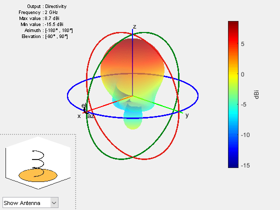
Plot the radiation pattern of a helix antenna with transparency specified as 0.5.

p = PatternPlotOptions
p = 
  PatternPlotOptions with properties:

      Transparency: 1
         SizeRatio: 0.9000
    MagnitudeScale: []
     AntennaOffset: [0 0 0]

p.Transparency = 0.5;
ant = helix;
pattern(ant,2e9,patternOptions=p)

Figure contains 2 axes objects and other objects of type uicontrol. Axes object 1 contains 4 objects of type patch, surface. Hidden axes object 2 contains 17 objects of type surface, line, text, patch.

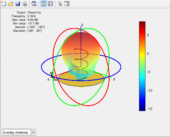
To understand the effect of Transparency, chose Overlay Antenna in the radiation pattern plot.

This option overlays the helix antenna on the radiation pattern.

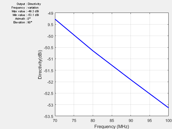
Plot radiation pattern of dipole antenna in rectangular cartesian co-ordinate system.

pattern(dipole, 70e6:10e6:100e6, 0, 90, CoordinateSystem="rectangular")

Figure contains an axes object and other objects of type uicontrol. The axes object with xlabel Frequency (MHz), ylabel Directivity(dBi) contains an object of type line.

View the directivity values at 0° azimuth and 90° elevation.

D = pattern(dipole, 70e6:10e6:100e6, 0, 90, CoordinateSystem="rectangular")
D = 4×1

  -49.5701
  -50.5630
  -50.3854
  -49.1831

Visualize gain plot of radial monopole antenna.

pattern(monopoleRadial,75e6,Type="gain")

Figure contains 2 axes objects and other objects of type uicontrol. Axes object 1 contains 5 objects of type patch, surface. Hidden axes object 2 contains 17 objects of type surface, line, text, patch.

Visualize gain plot of radial monopole antenna.

pattern(monopoleRadial,75e6,Type="realizedgain")

Figure contains 2 axes objects and other objects of type uicontrol. Axes object 1 contains 5 objects of type patch, surface. Hidden axes object 2 contains 17 objects of type surface, line, text, patch.

Input Arguments

collapse all

Antenna or array from catalog, custom antenna or array, installed antenna on a platform, or measured antenna object, specified as an object.

Example: yagiUda

Frequency to calculate or plot the antenna or array radiation pattern, specified as a scalar or a vector in Hz. The vector frequencies support rectangular coordinate system.

Example: 70e6

Data Types: double

Azimuth angles and spacing between the angles to visualize the radiation pattern, specified as a vector in degrees. If the coordinate system is set to uv, then the U values are specified in this parameter. The values of U are between -1 to 1.

Example: 90

Data Types: double

Elevation angles and spacing between the angles to visualize the radiation pattern, specified as a vector in degrees. If the coordinate system is set to uv, then the V values are specified in this parameter. The values of V are between -1 to 1.

Example: 0:1:360

Data Types: double

Name-Value Arguments

Specify optional pairs of arguments as Name1=Value1,...,NameN=ValueN, where Name is the argument name and Value is the corresponding value. Name-value arguments must appear after other arguments, but the order of the pairs does not matter.

Example: CoordinateSystem="uv"

Before R2021a, use commas to separate each name and value, and enclose Name in quotes.

Example: 'CoordinateSystem','uv'

Coordinate system to visualize the radiation pattern, specified as a string from one of these: "polar", "rectangular", "uv".

Example: "rectangular"

Data Types: string

Quantity to plot, specified as a string from one of these:

  • directivity – Directivity in dBi

  • gain – Gain in dBi

    Note

    The antenna Gain and Directivity are measured at a distance of 100λ.

  • realizedgain – Realized gain in dBi

  • efield – Electric field in Volt/meter

  • power – Power in (Volt/meter)2

  • powerdb – Power in dB

  • phase – Phase in degrees

    Note

    Type can only be set to phase when Polarization is provided.

The default value is "directivity" for a lossless antenna and "gain" for a lossy antenna. You cannot plot the "directivity" of a lossy antenna. For a detailed explanation on types and polarization, see Field Calculation in Antennas

Example: "efield"

Data Types: string

Flag to enable or disable field pattern normalization, specified as either true or false.

Example: false

Data Types: logical

2-D pattern display style when frequency is a vector, specified as a string from one of these:

  • overlay – Overlay frequency data in a 2-D line plot

  • waterfall – Plot frequency data in a waterfall plot

You can use this property when using pattern function without any output arguments.

Example: "waterfall"

Data Types: string

Field polarization, specified as a string from one of these:

  • H – Horizontal polarization

  • V – Vertical polarization

  • RHCP – Right-hand circular polarization

  • LHCP – Left-hand circular polarization

By default, you can visualize a combined polarization.

Example: "RHCP"

Data Types: string

Antenna element in array, specified as a scalar. This antenna element is connected to the voltage source.

Note

Use this property to calculate the embedded pattern of an array.

Example: 1

Data Types: double

Impedance value for array element termination, specified as a scalar. The impedance value terminates other antenna elements of an array while calculating the embedded pattern of the antenna connected to the voltage source.

Note

Use this property to calculate the embedded pattern of an array.

Example: 40

Data Types: double

Parameter to change pattern plot properties, specified as a PatternPlotOptions output. The input arguments that you can vary are:

  • Transparency

  • SizeRatio

  • AntennaOffset

  • MagnitudeScale

Example: PatternPlotOptions(Transparency=0.1)

Data Types: double

Output Arguments

collapse all

Radiation pattern of antenna or array or embedded pattern of array, returned as a matrix of number of elevation values by number of azimuth values. The pattern is one of the following:

  • directivity – Directivity in dBi (lossless antenna or array)

  • gain – Gain in dBi (lossy antenna or array)

  • realizedgain – Realized gain in dBi (lossy antenna or array)

  • efield – Electric field in volt/meter

  • power – Power in (Volt/meter)2

  • powerdb – Power in dB

Matrix size is number of elevation values multiplied by number of azimuth values.

Note

For more information, refer Field Calculation in Antennas.

Data Types: double

Azimuth angles to calculate the radiation pattern, returned as a vector in degrees.

Data Types: double

Elevation angles to calculate the radiation pattern, returned as a vector in degrees.

Data Types: double

References

[1] Makarov, Sergey N. Antenna and EM Modeling in MATLAB. Chapter3, Sec 3.4 3.8. Wiley Inter-Science.

[2] Balanis, C.A. Antenna Theory, Analysis and Design, Chapter 2, sec 2.3-2.6, Wiley.

Version History

Introduced in R2015a