plot
Display RF propagation rays in Site Viewer
Description
plot(
displays the rays using additional options specified by name-value arguments.rays,Name=Value)
Examples
Perform ray tracing in Chicago and return the rays in comm.Ray objects. Then, display the rays without performing the ray tracing analysis again.
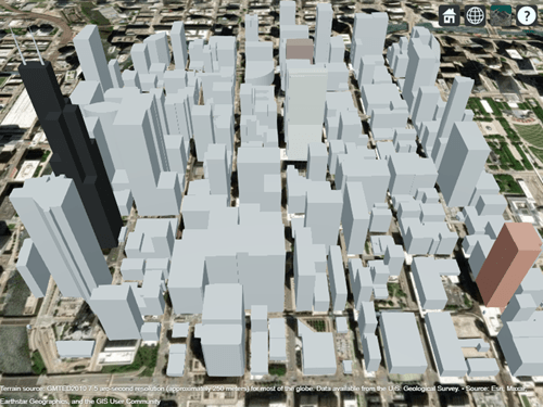
Launch Site Viewer with buildings in Chicago. For more information about the OpenStreetMap® file, see [1].
viewer = siteviewer(Buildings="chicago.osm");
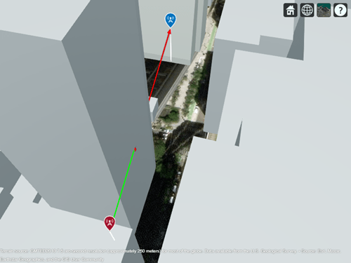
Create a transmitter site on one building and a receiver site on another building. Show the line-of-sight path between the sites using the los function.
tx = txsite(Latitude=41.8800, ...
    Longitude=-87.6295, ...
    TransmitterFrequency=2.5e9);
rx = rxsite(Latitude=41.881352, ...
    Longitude=-87.629771, ...
    AntennaHeight=30);
los(tx,rx)

Create a ray tracing propagation model, which MATLAB® represents using a RayTracing object. By default, the model uses the SBR method and calculates propagation paths with up to two reflections.
pm = propagationModel("raytracing");Perform the ray tracing analysis. The raytrace function returns a cell array containing the comm.Ray objects.
rays = raytrace(tx,rx,pm)
rays = 1×1 cell array
    {1×3 comm.Ray}
View the properties of the first ray object.
rays{1}(1)ans =
Ray with properties:
PathSpecification: 'Locations'
CoordinateSystem: 'Geographic'
TransmitterLocation: [3×1 double]
ReceiverLocation: [3×1 double]
LineOfSight: 0
Interactions: [1×1 struct]
Frequency: 2.5000e+09
PathLossSource: 'Custom'
PathLoss: 92.7686
PhaseShift: 1.2945
Read-only properties:
PropagationDelay: 5.7088e-07
PropagationDistance: 171.1462
AngleOfDeparture: [2×1 double]
AngleOfArrival: [2×1 double]
NumInteractions: 1
Close Site Viewer.
close(viewer)
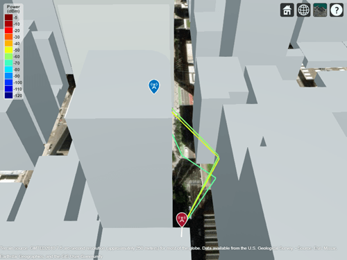
Create another Site Viewer with the same buildings, transmitter site, and receiver site. Then, display the propagation paths. Alternatively, you can plot individual paths by specifying a single ray object, for example rays{1}(2).
siteviewer(Buildings="chicago.osm");
show(tx)
show(rx)
plot(rays{1},Type="power", ...
    TransmitterSite=tx,ReceiverSite=rx)

Appendix
[1] The OpenStreetMap file is downloaded from https://www.openstreetmap.org, which provides access to crowd-sourced map data all over the world. The data is licensed under the Open Data Commons Open Database License (ODbL), https://opendatacommons.org/licenses/odbl/.
Input Arguments
Propagation rays, specified as a comm.Ray object or a
vector of comm.Ray objects. The PathSpecification
property of the ray must be "Locations".
Name-Value Arguments
Specify optional pairs of arguments as
Name1=Value1,...,NameN=ValueN, where Name is
the argument name and Value is the corresponding value.
Name-value arguments must appear after other arguments, but the order of the
pairs does not matter.
Example: plot(rays,Type="pathloss",ColorLimits=[-100 0]) adjusts the
default color limits of the plotted ray.
Before R2021a, use commas to separate each name and value, and enclose
Name in quotes.
Example: plot(rays,"Type","pathloss","ColorLimits",[-100 0]) adjusts
the default color limits of the plotted ray.
Type of quantity to plot, specified as one of these options:
"pathloss"— The color of the path indicates the path loss in dB."power"— The color of the path indicates the power of the signal in dBm.
Data Types: char | string
Color limits for the colormap, specified as a 1-by-2 vector of the form
[cmin cmax]. The value of cmin must be less
than the value of cmax. cmin represents the
lower saturation limit and cmax represents the upper saturation
limit.
The default value is [-120 -5] when Type
is "power" and [45 160] when
Type is "pathloss".
Data Types: double
Colormap for the propagation paths, specified as a colormap name or as an M-by-3 array of RGB triplets that define M individual colors.
This table lists the colormap names.
| Colormap Name | Color Scale |
|---|---|
|
|
|
|
|
|
|
|
|
|
|
|
|
|
|
|
|
|
|
|
|
|
|
|
|
|
|
|
|
|
|
|
|
|
|
|
|
|
|
|
|
|
|
|
Data Types: double | char | string
Show the color legend on the map, specified as true or
false.
Data Types: logical
Map for visualization and surface data, specified as a siteviewer
object.1
By default, the function displays the rays in the current
siteviewer object or a new siteviewer object if
none are open.
Version History
Introduced in R2020aWhen you display propagation rays created from a RayTracing propagation
model object with custom materials, the information box in Site Viewer reports these
material names:
"custom-buildings-material", for a custom buildings material specified using theBuildingsMaterialproperty of theRayTracingobject."custom-terrain-material", for a custom terrain material specified using theTerrainMaterialproperty of theRayTracingobject."custom-surface-material", for a custom surface material specified using theSurfaceMaterialproperty of theRayTracingobject.
In previous releases, the information box displays names such as
"custom1" and "custom2".
1 Alignment of boundaries and region labels are a presentation of the feature provided by the data vendors and do not imply endorsement by MathWorks®.
MATLAB Command
You clicked a link that corresponds to this MATLAB command:
Run the command by entering it in the MATLAB Command Window. Web browsers do not support MATLAB commands.
选择网站
选择网站以获取翻译的可用内容,以及查看当地活动和优惠。根据您的位置,我们建议您选择:。
您也可以从以下列表中选择网站:
如何获得最佳网站性能
选择中国网站(中文或英文)以获得最佳网站性能。其他 MathWorks 国家/地区网站并未针对您所在位置的访问进行优化。
美洲
- América Latina (Español)
- Canada (English)
- United States (English)
欧洲
- Belgium (English)
- Denmark (English)
- Deutschland (Deutsch)
- España (Español)
- Finland (English)
- France (Français)
- Ireland (English)
- Italia (Italiano)
- Luxembourg (English)
- Netherlands (English)
- Norway (English)
- Österreich (Deutsch)
- Portugal (English)
- Sweden (English)
- Switzerland
- United Kingdom (English)