Antenna Array Analysis
This example shows how to create and analyze antenna arrays in Antenna Toolbox™, with emphasis on concepts such as beam scanning, sidelobe level, mutual coupling, element patterns, and grating lobes. The analyses is performed on a 9-element linear array of half-wavelength dipoles.
Design Frequency and Array parameters
Choose the design frequency to be 1.8 GHz, which happens to be one of the carrier frequencies for 3G/4G cellular systems. Define array size using number of elements, N and inter-element spacing, dx.
freq = 1.8e9;
c = physconst("lightspeed");
lambda = c/freq;
N = 9;
dx = 0.49*lambda;
Create Resonant Dipole
The individual element of the array is a dipole. The initial length of this dipole is chosen to be . Trim its length so as to achieve resonance (X~0 ).
dipole_L = lambda/2;
dipole_W = lambda/200;
mydipole = dipole;
mydipole.Length = dipole_L;
mydipole.Width = dipole_W;
mydipole.TiltAxis = "Z";
mydipole.Tilt = 90;
fmin = freq - .05*freq;
fmax = freq + .05*freq;
minX = 0.0001;          % Minimum value of reactance to achieve
trim = 0.0005;          % The amount to shorten the length at each iteration
resonant_dipole = dipole_tuner(mydipole,freq,fmin,fmax,minX,trim);
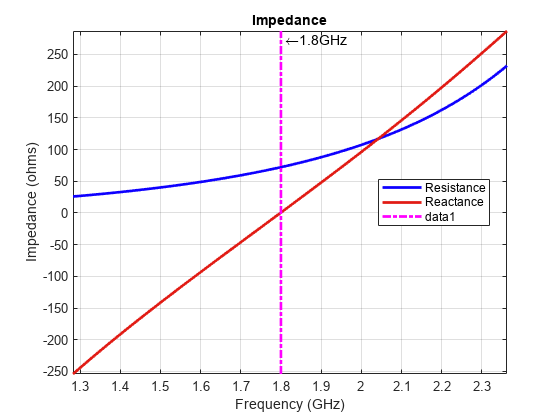
Z_resonant_dipole = impedance(resonant_dipole,freq)
Z_resonant_dipole =
71.8451 - 0.3691i
helement = figure;
show(resonant_dipole)
axis tight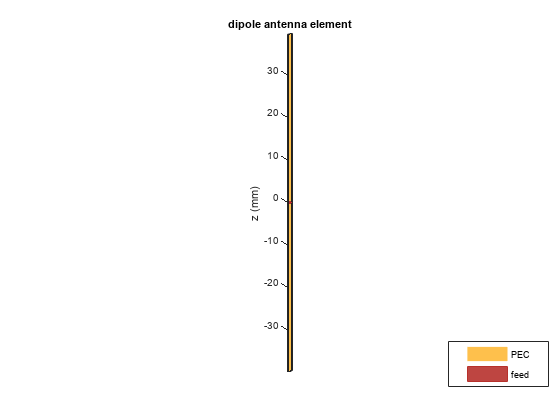
Create Linear Array
Assign the resonant dipole as the individual radiator of a linear array. While the isolated dipole has been tuned for resonance at the design frequency, it will get detuned in the array environment. Modify the number of elements and spacing and observe the array geometry. The elements are positioned on the x-axis and are numbered from left to right.
dipole_array = linearArray;
dipole_array.Element = resonant_dipole;
dipole_array.NumElements = N;
dipole_array.ElementSpacing = dx;
hArray = figure;
show(dipole_array)
axis tight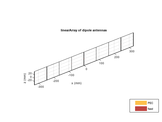
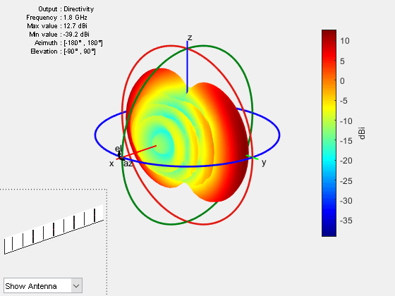
Plot 3-D Array Pattern
Visualize the pattern for the linear array in 3-D space at the design frequency.
pattern3Dfig = figure;
pattern(dipole_array,freq)
Plot 2-D Radiation Pattern
The 3-D pattern of the array shows the maximum of the beam at an azimuthal angle of 90 deg. Plot the 2-D radiation pattern in the azimuthal plane(x-y plane) which corresponds to zero elevation angle.
patternazfig1 = figure;
az_angle = 1:0.25:180;
pattern(dipole_array,freq,az_angle,0,CoordinateSystem="rectangular")
axis([0 180 -25 15])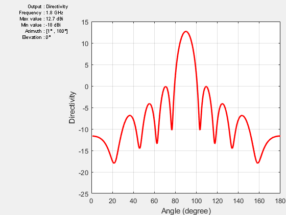
The array has a peak directivity of 12.83 dBi, and the first sidelobes on either side of the peak are approximately 13 dB down. This is because the array has a uniform amplitude taper with all elements fed at 1V. The sidelobe level can be controlled by using different amplitude tapers on the array elements such as Chebyshev and Taylor.
Beam Scanning
Choosing a set of phase shifts allows us to scan the beam to a specific angle. This linear array configuration enables scanning in the azimuthal plane (x-y plane), which corresponds to zero elevation angle. Scan the beam 30 deg off broadside (azimuthal angle of 120 deg).
scanangle = [120 0];
ps = phaseshift(freq,dx,scanangle,N);
dipole_array.PhaseShift = ps;
patternazfig2 = figure;
pattern(dipole_array,freq,az_angle,0,CoordinateSystem="rectangular")
axis([0 180 -25 15])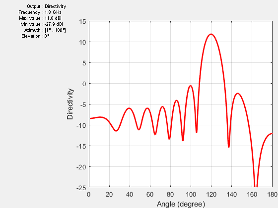
The peak of the main beam is now 30 deg away from the initial peak (azimuth = 90 deg). Note the drop in directivity of about 0.9 dB. For infinite arrays, this drop increases with increasing the scan angle according to a cosine law.
Plot Element Patterns of Corner and Central Elements
In small arrays, the pattern of the individual element can vary significantly. In order to establish this fact, plot the pattern of the central elements and of the two edge elements. To obtain these patterns, excite every element alone and terminate the rest into a reference impedance. The elements are numbered from left to right, in the direction of the x-axis.
element_number = [1 ceil(N/2)-1 ceil(N/2) ceil(N/2)+1 N];
D_element = nan(numel(element_number),numel(az_angle));
legend_string = cell(1,numel(element_number));
for i = 1:numel(element_number)
    D_element(i,:) = pattern(dipole_array,freq,az_angle,0, ...
                           CoordinateSystem="rectangular", ...
                           ElementNumber=element_number(i), ...
                           Termination=real(Z_resonant_dipole));
    legend_string{i} = strcat('N = ',num2str(element_number(i)));
end
patternazfig3 = figure;
plot(az_angle,D_element,LineWidth=1.5)
xlabel("Azimuth (deg)")
ylabel("Directivity (dBi)")
title("Element Patterns")
grid on
legend(legend_string,Location="best")
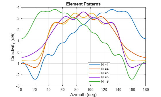
The plot of the element patterns reveals that, apart from the central element, all the others are mirror images about the center of the plot, i.e. the element pattern of the 1st element is a mirror reflection about azimuth = 90 deg of the element pattern of the 9th element, etc.
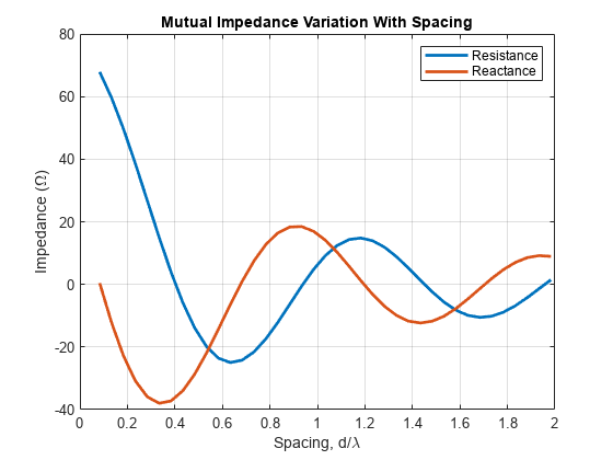
Mutual Coupling
Mutual coupling is the phenomenon whereby currents developed on each element in the array do not depend only on their own excitation, but have contributions from other elements as well. To study this effect, we will simplify the array to a 2-element case similar to [1].
dipole_array.NumElements = 2;
dipole_array.AmplitudeTaper = 1;
dipole_array.PhaseShift = 0;
To observe the effect of mutual coupling, vary the spacing between the array elements and plot the variation in , mutual impedance between the pair of dipoles in the array [1]. Since the elements are parallel to each other, the coupling is strong.
spacing = (lambda/2:0.05:2).*lambda;
Z12 = nan(1,numel(spacing));
for i = 1:numel(spacing)
    dipole_array.ElementSpacing = spacing(i);
    s = sparameters(dipole_array,freq,real(Z_resonant_dipole));
    S = s.Parameters;
    Z12(i) = 2*S(1,2)*70/((1 - S(1,1))*(1- S(2,2)) - S(1,2)*S(2,1));
end
mutualZ12fig = figure;
plot(spacing./lambda,real(Z12),spacing./lambda,imag(Z12),LineWidth=2)
xlabel("Spacing, d/\lambda")
ylabel("Impedance (\Omega)")
grid on
title("Mutual Impedance Variation With Spacing")
legend("Resistance","Reactance")
Grating Lobes
Grating lobes are the maxima of the main beam predicted by the pattern multiplication theorem. When the array spacing is less than or equal to , only the main lobe exists in the visible space with no other grating lobes. Grating lobes appear when the array spacing is greater than . For large spacing, grating lobe(s) could appear in the visible space even at zero scan angle. Investigate grating lobes for a linear array of 9 dipoles. Scan the beam 0 deg off broadside (azimuthal angle of 90 deg).
dipole_array.NumElements = 9;
dipole_array.ElementSpacing = lambda/2;
D_half_lambda = pattern(dipole_array,freq,az_angle,0,CoordinateSystem="rectangular");
dipole_array.ElementSpacing = 0.75*lambda;
D_three_quarter_lambda = pattern(dipole_array,freq,az_angle,0,CoordinateSystem="rectangular");
dipole_array.ElementSpacing = 1.5*lambda;
D_lambda = pattern(dipole_array,freq,az_angle,0,CoordinateSystem="rectangular");
patterngrating1 = figure;
plot(az_angle,D_half_lambda,az_angle,D_three_quarter_lambda,az_angle,D_lambda,LineWidth=1.5);
grid on
xlabel("Azimuth (deg)")
ylabel("Directivity (dBi)")
title("Array Pattern (Elevation = 0 deg)")
legend("d=\lambda/2","d=0.75\lambda","d=1.5\lambda",Location="best")
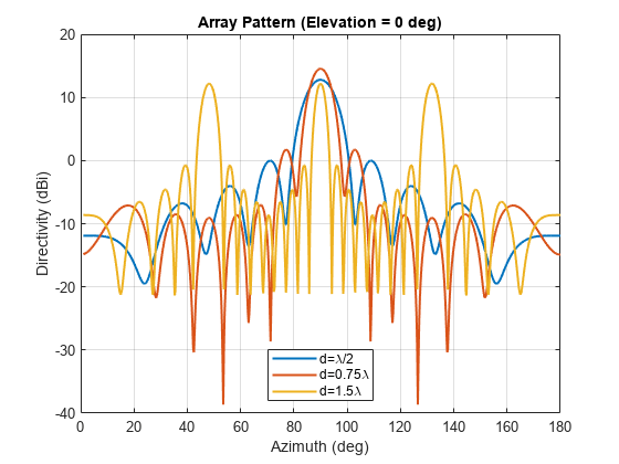
Compared to the spaced array, the spaced array shows 2 additional equally strong peaks in the visible space - the grating lobes. The spaced array still has a single unique beam peak at zero scan off broadside (azimuthal angle of 90 deg). Scan this array off broadside to observe appearance of the grating lobes.
dipole_array.ElementSpacing = 0.75*lambda;
azscan = 45:10:135;
scanangle = [azscan ;zeros(1,numel(azscan))];
D_scan = nan(numel(azscan),numel(az_angle));
legend_string1 = cell(1,numel(azscan));
for i = 1:numel(azscan)
    ps = phaseshift(freq,dx,scanangle(:,i),N);
    dipole_array.PhaseShift = ps;
    D_scan(i,:) = pattern(dipole_array,freq,az_angle,0,CoordinateSystem="rectangular");
    legend_string1{i} = strcat('scan = ',num2str(azscan(i)),' deg');
end
patterngrating2 = figure;
plot(az_angle,D_scan,LineWidth=1)
xlabel("Azimuth (deg)")
ylabel("Directivity (dBi)")
title("Scan Pattern for 0.75\lambda Spacing Array ((Elevation = 0 deg)")
grid on
legend(legend_string1,Location="best")
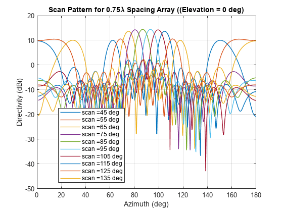
The spacing array with uniform excitation and zero phaseshift does not have grating lobes in the visible space. The peak of the main beam occurs at broadside (azimuth = 90 deg). However for the scan angle of 65 deg and lower, and for 115 deg and higher the grating lobe enters visible space. To avoid grating lobes, choose an element spacing of or less. With smaller spacing, the mutual coupling is stronger.
Effect of Element Pattern on Array Pattern
To study the effect of the element pattern on the overall array pattern, plot the normalized central element pattern versus the normalized directivity of the linear array of 9 dipoles at broadside.
dipole_array.ElementSpacing = 0.49*lambda;
dipole_array.PhaseShift = 0;
Dmax = pattern(dipole_array,freq,90,0);
D_scan = nan(numel(azscan),numel(az_angle));       % Pre-allocate
legend_string2 = cell(1,numel(azscan)+1);
legend_string2{1} = 'Center element';
for i = 1:numel(azscan)
    ps = phaseshift(freq,dx,scanangle(:,i),N);
    dipole_array.PhaseShift = ps;
    D_scan(i,:) = pattern(dipole_array,freq,az_angle,0,CoordinateSystem="rectangular");
    D_scan(i,:) = D_scan(i,:) - Dmax;
    legend_string2{i+1} = strcat('scan = ',num2str(azscan(i)));
end
patternArrayVsElement = figure;
plot(az_angle,D_element(3,:) - max(D_element(3,:)),LineWidth=3)
hold on
plot(az_angle,D_scan,LineWidth=1)
axis([min(az_angle) max(az_angle) -20 0])
xlabel("Azimuth (deg)")
ylabel("Directivity (dBi)")
title("Scan Pattern for 0.49\lambda Spacing Array")
grid on
legend(legend_string2,Location="southeast")
hold off
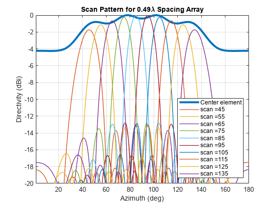
Note the overall shape of the normalized array pattern approximately follows the normalized central element pattern close to broadside. The array pattern in general is the product of the element pattern and the array factor (AF).
Reference
[1] W. L. Stutzman, G. A. Thiele, Antenna Theory and Design, p. 307, Wiley, 3rd Edition, 2013.