Design and Analysis of Compact Ultra-Wideband MIMO Antenna Array

Create Upper Patches and Feed Lines of Monopole Antennas

The MIMO array consists of two orthogonal planar monopole antennas lying in the horizontal plane. The size of the upper conductor of each monopole antenna is 10 mm by 16 mm. The size of the conductor-backed dielectric substrate is 40 mm by 26 mm. The square radiator of the first monopole is offset by 7 mm, 14 mm, and 0 mm in the x-, y-, and z-directions, respectively, from one of the corners of the substrate. The second monopole radiator is offset by 14 mm, 9 mm, and 0 mm in the x-, y-, and z-directions, respectively, from the diagonally opposite corner of the substrate.

Define the geometry of the first monopole radiator and create the antenna using the antenna.Rectangle object.

lp = 10e-3;
xg = 40e-3;
yg = 26e-3;
px1 = -xg/2 + 7e-3; 
py1 = -yg/2 + 14e-3;
patch1 = antenna.Rectangle(Center=[px1 py1],Length=lp,Width=lp);

Define the geometry of the second monopole radiator and create the antenna using the antenna.Rectangle object.

px2 = xg/2 - 9e-3 - lp/2;
py2 = yg/2 - 8.1e-3 - 0.9e-3;
patch2 = antenna.Rectangle(Center=[px2 py2],Length=lp,Width=lp);

Feed both monopole antennas using two orthogonally oriented identical planar feedlines with a length and width of 9 mm and 1.8 mm, respectively.

feed1 = antenna.Rectangle(Center=[px1 py1-lp/2-9e-3/2],Length=1.8e-3,Width=9e-3);
feed2 = antenna.Rectangle(Center=[px2+lp/2+9e-3/2 py2],Length=9e-3,Width=1.8e-3);

Create and Visualize Upper Layer

Join the patches to create the upper layer of the MIMO array which consists of two square radiators and two feed lines of the monopole antennas. Use the show function to visualize the uppermost layer of the array.

patchUpper = patch1 + patch2 + feed1 + feed2;
figure
show(patchUpper)

Create and Visualize Ground Layer

The ground layer consists of two rectangular shapes, two rectangular slots and three stubs. The purposes of introducing this perturbation in the ground plane are to achieve good impedance matching across the entire frequency band and to minimize the mutual coupling between the monopole antennas of the MIMO array.

Create the left rectangular ground block.

ground1 = antenna.Rectangle(Center=[-xg/2+29e-3/2 -yg/2+4e-3],Length=29e-3,Width=8e-3);

Slot in the left rectangular ground block.

groundcut1 = antenna.Rectangle(Center=[-xg/2+5e-3+4e-3/2 -yg/2+8e-3-1e-3/2],Length=4e-3,Width=1e-3);

Create the left ground plane by subtracting the slot from the ground in the left ground block.

ground1 = ground1 - groundcut1;

Create the left rectangular ground block.

ground2 = antenna.Rectangle(Center=[xg/2-4e-3 0],Length=8e-3,Width=26e-3);

Slot in the right rectangular ground block.

groundcut2 = antenna.Rectangle(Center=[xg/2-8e-3+1e-3/2 py2],Length=1e-3,Width=4e-3);

Create the left ground plane by subtracting the slot from the ground in the left ground block.

ground2 = ground2 - groundcut2;

Create the ground interconnection.

ground3 = antenna.Rectangle(Center=[xg/2-8e-3-3e-3/2 -yg/2+1e-3/2],Length=3e-3,Width=1e-3);

Connect the three ground blocks.

ground = ground1 + ground2 + ground3;

Create the ground stubs.

groundstub1 = antenna.Rectangle(Center=[-xg/2+14e-3+1e-3/2 yg/2-18e-3/2],Length=1e-3,Width=18e-3);
groundstub2 = antenna.Rectangle(Center=[-xg/2+14e-3-5e-3/2 yg/2-1e-3/2],Length=5e-3,Width=1e-3);
groundstub3 = antenna.Rectangle(Center=[xg/2-8e-3+1e-3-16e-3/2 yg/2-16e-3-1e-3/2],Length=16e-3,Width=1e-3);

Connect all the stubs with the ground block and display the result.

ground = ground + groundstub1 + groundstub2 + groundstub3;
figure
show(ground)

Assign Dielectric Properties and Excite Antennas

Design the entire MIMO array on a dielectric substrate with relative permittivity and loss tangent values of 3.5 and 0.004, respectively. Set the thickness of the dielectric substrate to 0.8 mm.

h = 0.8e-3;
d = dielectric(EpsilonR=3.5,...
    LossTangent=0.004,Thickness=h);

Create a pcbStack object using the same dielectric substrate. Assign patchUpper and ground to the upper and lower layers of the pcbStack object, respectively.

ps = pcbStack;
ps.BoardThickness = h;
r1bottom = antenna.Rectangle(Center=[0,0],Length=xg,Width=yg);
ps.BoardShape = r1bottom;
ps.Layers = {patchUpper,d,ground};

Define feed locations at the edge of each antenna feed line. Set the feed diameter to half of the feedline width. Excite each antenna with a unit amplitude and zero phase voltage source.

fx1 = -xg/2 + 6.1e-3 + 1.8e-3/2;
fy1 = -yg/2;
fx2 = xg/2;
fy2 = yg/2 - 8.1e-3 - 1.8e-3/2;
ps.FeedLocations = [fx1 fy1 1 3; fx2 fy2 1 3];
ps.FeedDiameter = 1.8e-3/2;
ps.FeedVoltage = [1 1];
ps.FeedPhase = [0 0];

Visualize S-Parameters of Array

Manually mesh the array geometry with a maximum edge length of 1.4 mm.

ax = figure;
mesh(ps,MaxEdgeLength=1.4e-3)

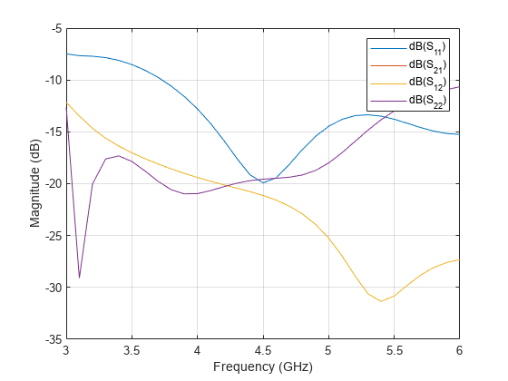
Use the sparameters function to calculate the scattering parameters of the array. Because the array has two ports, it has four S-parameters. ${\mathit{S}}_{11}$ and ${\mathit{S}}_{22}$ represent the reflection coefficient at ports 1 and 2, respectively. ${\mathit{S}}_{12}$ and ${\mathit{S}}_{21}$ characterize the mutual coupling between the ports. Use the rfplot function to visualize the port parameters. Due to the large number of basis functions, simulating the frequency variation can take several minutes. By default, simulation of the frequency variation is disabled and the results are from a precomputed model. To enable simulation of the frequency variation, set runModel to true.

Define the frequency range in Hz.

f1 = linspace(3,6,31)*1e9;
runModel = false;

Compute the S-parameters.

if runModel
        s = sparameters(ps,f1);
    else
        load("frequencyVariationData.mat")  
end

Plot the S-parameters.

figure
rfplot(s)

Plot Directivity, Gain, and Realized Gain Patterns with Both Excitations

Use the pattern function to visualize different radiation patterns of the array with excitation in both antennas.You can configure this function to calculate the directivity, gain, or realized gain pattern. By default, the function computes the directivity for a lossless antenna and the gain for a lossy antenna.

The directivity is the ratio of the radiation intensity in a specific angular direction to the average radiated power. Directivity does not depend on material loss or impedance mismatch. The gain is the product of the directivity and radiation efficiency. The radiation efficiency is the ratio of the total radiated power to the total input power going into the antenna or array input ports.

The material losses, such as finite conduction loss and dielectric loss, are accounted in the radiation efficiency and gain parameter. As part of a complete RF system, antennas and arrays are commonly connected with an impedance-matching network. The impedance mismatch of the antenna or array with this network leads to a finite port mismatch loss, which is characterized by the port efficiency. Port efficiency is the ratio of the input power provided by the external excitation ports and the power received at the antenna or array input feeding edges. The realized gain is the product of the gain and the port efficiency. Directivity, gain, and realized gain patterns of the MIMO array at 3 GHz are as below. The gain is lower than the directivity because the radiation efficiency is less than 1. Similarly, the realized gain is lower than the gain value due to finite impedance mismatch loss.

figure
pattern(ps,3e9,'Type','directivity');

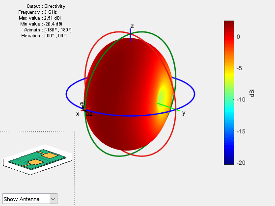
figure
pattern(ps,3e9,'Type','gain');

figure
pattern(ps,3e9,'Type','realizedgain');

Use the efficiency function to calculate the radiation efficiency of the array.

e = efficiency(ps,3e9)

e = 
0.9740

Visualize Directivity, Gain, and Realized Gain Patterns with Single Excitation

Configure the scenario from [1] in which, only one antenna of the array is excited and the other is shorted by setting the FeedVoltage and FeedPhase properties such that only the first antenna is excited.

ps.FeedVoltage = [1 0];
ps.FeedPhase = [0 0];

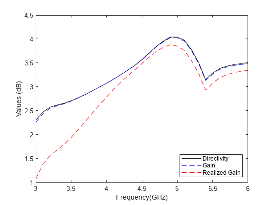
Compute and plot the directivity, gain, and realized gain values over a broad frequency range. The gain values increase with the frequency up to approximately 5 GHz, which indicates that the array radiation pattern becomes more directional as frequency increases to that point.

if runModel
    for m=1:length(f1)
        patD1 = pattern(ps,f1(m),'Type','directivity');
        patG1 = pattern(ps,f1(m),'Type','gain');
        patRG1 = pattern(ps,f1(m),'Type','realizedgain');
        D1(1,m) = max(max(patD1));
        G1(1,m) = max(max(patG1));
        RG1(1,m) = max(max(patRG1));
    end
end
figure
plot(f1./1e9,D1,"k")
hold on
plot(f1./1e9,G1,"--b")
plot(f1./1e9,RG1,"--r")
xlabel("Frequency(GHz)")
ylabel("Values (dB)")
legend("Directivity","Gain","Realized Gain",Location="southeast")

Conclusion

This example shows how to efficiently design an advanced complex PCB antenna array and evaluate its impedance and radiation characteristics.

References

[1] L. Liu, S. W. Cheung, T. I. Yuk and D. Wu. "A Compact Ultrawideband MIMO Antenna," 2013 7th European Conference on Antennas and Propagation (EuCAP), Sweden, 2013.