Impedance Matching of Non-resonant (Small) Monopole
This example shows how to design a double tuning L-section matching network between a resistive source and capacitive load in the form of a small monopole. The L-section consists of two inductors. The network achieves conjugate match and guarantees maximum power transfer at a single frequency.
Create Monopole
Create a quarter-wavelength monopole antenna with the resonant frequency around 1 GHz. For the purpose of this example, we choose a square ground plane of side .
fres = 1e9;
speedOfLight = physconst("lightspeed");
lambda = speedOfLight/fres;
L = 0.25*lambda;
dp = monopole(Height=L,Width=L/50,...
    GroundPlaneLength=0.75*lambda,GroundPlaneWidth=0.75*lambda);
Calculate Monopole Impedance
Specify the source (generator) impedance, the reference (transmission line) impedance and the load (antenna) impedance. In this example, the load Zl0 will be the non-resonant (small) monopole at the frequency of 500 MHz, which is the half of the resonant frequency. The source has the equivalent impedance of 50 ohms.
f0 = fres/2;
Zs = 50;
Z0 = 50;
Zl0 = impedance(dp,f0);
Rl0 = real(Zl0);
Xl0 = imag(Zl0);
Define the number of frequency points for the analysis and a frequency band centered at 500 MHz.
Npts = 30;
fspan = 0.1;
fmin = f0*(1 - (fspan/2));
fmax = f0*(1 + (fspan/2));
freq = unique([f0 linspace(fmin,fmax,Npts)]);
Understand Load Behavior using Reflection Coefficient and Power Gain
Calculate the load reflection coefficient and the power gain between the source and the antenna.
S = sparameters(dp, freq);
GammaL = rfparam(S,1,1);
Gt = 10*log10(1 - abs(GammaL).^2);
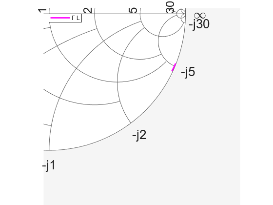
Plotting the input reflection coefficient on a Smith chart shows the capacitive behavior of this antenna around the operating frequency of 500 MHz. The center of the Smith chart represents the matched condition to the reference impedance. The location of the reflection coefficient trace around confirms that there is a severe impedance mismatch.
fig1 = figure;
hsm = smithplot(fig1,freq,GammaL,LineWidth=2.0,Color='m',...
    View="bottom-right",LegendLabels={'#Gamma L'});
Plot the power delivered to the load.
fig2 = figure;
plot(freq*1e-6,Gt,'m',LineWidth=2);
grid on
xlabel("Frequency [MHz]")
ylabel("Magnitude (dB)")
title("Power delivered to load")
![Figure contains an axes object. The axes object with title Power delivered to load, xlabel Frequency [MHz], ylabel Magnitude (dB) contains an object of type line.](../../examples/antenna/win64/atx_nonresonant_monopole_match_02.png)
As the power gain plot shows, there is approximately a 20 dB power loss around the operating frequency (500 MHz).
Design Matching Network
The matching network must ensure maximum power transfer at 500 MHz. The L-section double tuning network achieves this goal [1]. The network topology, shown in the figure that follows consists of an inductor in series with the antenna, that cancels the large capacitance at 500 MHz, and a shunt inductor that further boosts the output resistance to match the source impedance of 50 .
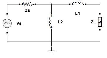
omega0 = 2*pi*f0;
L2 = (1/omega0)*sqrt((Zs*Rl0)/(1-(Rl0/Zs)));
L1 = (-Xl0/omega0) - (L2/2) - sqrt((L2^2/4)-(((Rl0)^2)/omega0^2));
Create Matching Network and Calculate S-parameters
The matching network circuit consists of two inductors whose inductance values have been calculated above. Create the matching network using the RF Toolbox™ and calculate the S-parameters of this network over the frequency band centered at the operating frequency.
IND1 = inductor(L1,'L1');
IND2 = inductor(L2,'L2');
MatchingNW = circuit("double_tuning");
add(MatchingNW,[0 1],IND2);
add(MatchingNW,[1 2],IND1);
setports(MatchingNW,[1 0],[2 0]);
Smatchnw = sparameters(MatchingNW,freq);
The circuit element representation of the matching network is shown below.
disp(MatchingNW)
  circuit: Circuit element

    ElementNames: {'L2'  'L1'}
        Elements: [1×2 inductor]
           Nodes: [0 1 2]
            Name: 'double_tuning'
Reflection Coefficient and Power Gain with Matching Network
Calculate the input reflection coefficient/power gain for the antenna load with the matching network.
Zl =  impedance(dp,freq);
GammaIn = gammain(Smatchnw,Zl);
Gtmatch = powergain(Smatchnw,Zs,Zl,'Gt');
Gtmatch = 10*log10(Gtmatch);
Compare Results
Plot the input reflection coefficient and power delivered to the antenna, with and without the matching network. The Smith chart plot shows the reflection coefficient trace going through its center thus confirming the match. At the operation frequency of 500 MHz, the generator transfers maximum power to the antenna. The match degrades on either side of the operating frequency.
add(hsm,freq,GammaIn);
hsm.LegendLabels(2) = {'#Gamma In'};
hsm.View = "full";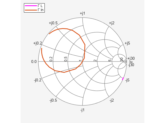
Plot the power delivered to the load.
figure(fig2)
hold on
plot(freq*1e-6,Gtmatch,LineWidth=2);
axis([min(freq)*1e-6,max(freq)*1e-6,-25,0])
legend("No matching network","Double tuning",Location="Best");
![Figure contains an axes object. The axes object with title Power delivered to load, xlabel Frequency [MHz], ylabel Magnitude (dB) contains 2 objects of type line. These objects represent No matching network, Double tuning.](../../examples/antenna/win64/atx_nonresonant_monopole_match_05.png)
References
[1] M. M. Weiner, Monopole Antennas, Marcel Dekker, Inc.,CRC Press, Rev. Exp edition, New York, pp.110-118, 2003.