Installed Antenna Analysis - Modelling Antennas with Platforms

Create a platform

The electrically large platform can be imported in Antenna Toolbox as an STL file. These STL files can be used to describe ships, planes or any other kind of structures on which the antenna element is mounted. In the present case the rectcavity.stl file is a large rectangular cavity created using the stlwrite function and then deleting the dipole antenna manually. h = cavity('Length', 4, 'Width', 1, 'Height', 0.5); z = impedance(h, 1e8); stlwrite(h, 'rectcavity.stl');

base = platform(FileName="rectcavity.stl", Units="m");
show(base);

Set-up the installed antenna analysis

The user defined platform can be specified in the installed antenna analysis. The user can choose the antenna element and its location with respect to the platform.

ant = installedAntenna;
ant.Platform = base;
show(ant);

Analyze the installed antenna setup

All the analysis that can be performed on the single antenna element can be performed in case of an installed antenna.

figure
impedance(ant,linspace(950e6,1050e6,51));

figure
pattern(ant,1e9);

To better visualize the current distribution on the platform it is better to select the log scale.

figure
current(ant,1e9,Scale="log");

Add multiple antennas on the platform

Installed antenna analysis can be performed with multiple antenna elements. In this case a rectangular patch microstrip antenna and a circular patch microstrip antenna are designed at 1 GHz and are placed inside the cavity structure 2 meters apart.

elem1 = design(patchMicrostrip,1e9);
elem2 = design(patchMicrostripCircular,1e9);
ant.ElementPosition = [-1 0 0.2; 1 0 0.2];
ant.Element = {elem1, elem2};
show(ant);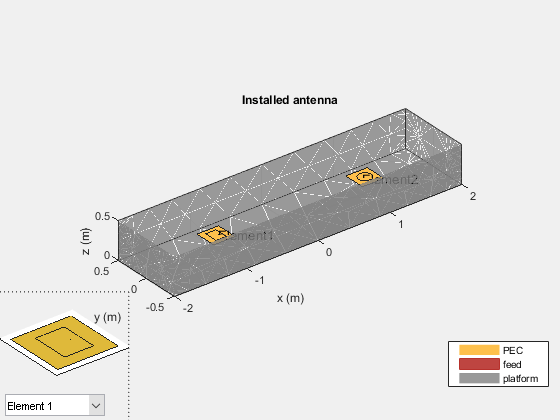

Analyze multiple antenna elements on a platform

All the analysis performed on a single antenna element can also be performed on multiple antenna elements.

figure
pattern(ant,1e9);

figure
current(ant,1e9,Scale="log");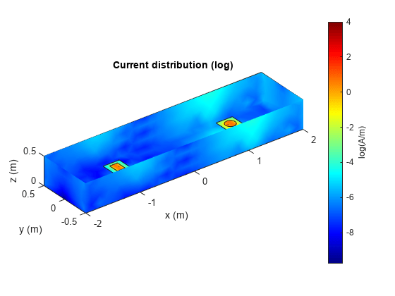

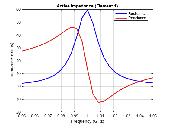
The plot below displays the impedance of the rectangular patch microstrip antenna.

figure
impedance(ant,linspace(950e6,1050e6,25),1);

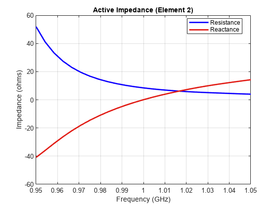
The plot below displays the impedance of the circular patch microstrip antenna.

figure
impedance(ant,linspace(950e6,1050e6,25),2);

The coupling between the antenna elements can be calculated using the s-parameters.

S = sparameters(ant,linspace(950e6,1050e6,25));
figure
rfplot(S);