ISM Band Microstrip Patch Antennas and Mutually Coupled Patches
This example shows how to design and analyze rectangular, circular, triangular and elliptical microstrip patch antennas operating in the ISM (Industrial Scientific and Medical) band 2.4 GHz - 2.5 GHz. In the second half, this example shows how to create an array of rectangular and triangular patch antennas, and gauge the effect of mutual coupling on its radiation pattern. This array configuration has lowest coupling among these ISM band patch antennas.
Define Parameters
All of these microstrip antennas are modeled on a 6.6 mm thick PCB having relative permittivity of 4.2, loss-tangent of 0.02, and square ground plane of 100 mm-by-100 mm. The PCB is fed by a coaxial probe of diameter 1.3 mm. Define the dimensions, dielectric material, and the analysis frequency range for these patch antennas.
lengthGp = 100e-3;
widthGp = 100e-3;
thickness = 6.6e-3;
d = dielectric(EpsilonR=4.2,LossTangent=0.02);
freq = 2.3e9:0.01e9:2.8e9;
Create Elliptical Patch Antenna
Create a probe-fed elliptical patch antenna with a 33.5 mm major axis, and a 18.8 mm minor axis of the patch. The feed is offset by 11.6 mm from the origin along the X-axis.
axisMajor = 33.5e-3;
axisMinor = 18.8e-3;
offset1 = 11.6e-3;
Use the patchMicrostripElliptical object to create this antenna using the defined parameters.
p_Elliptical = patchMicrostripElliptical(MajorAxis=axisMajor,MinorAxis=axisMinor,...
    Height=thickness,Substrate=d,GroundPlaneLength=lengthGp,...
    GroundPlaneWidth=widthGp,FeedOffset=[-(axisMajor/2-offset1) 0]);
figure
show(p_Elliptical)
title("Elliptical Patch Antenna");

Create Circular Patch Antenna
Create a probe-fed circular patch antenna with 16 mm patch radius. The feed is offset by 9.25 mm from the origin along the X-axis.
radius = 16e-3;
offset2 = 9.25e-3;
Use the patchMicrostripCircular object to create this antenna using the defined parameters.
p_Circular = patchMicrostripCircular(Radius=radius,Height=thickness,Substrate=d,...
    GroundPlaneLength=lengthGp,GroundPlaneWidth=widthGp,FeedOffset=[-(radius-offset2) 0]);
figure
show(p_Circular)
title("Circular Patch Antenna");

Create Rectangular Patch Antenna
Create a probe-fed rectangular patch antenna with 28.20 mm patch length, and 34.06 mm patch width. The feed is offset by 5.3 mm from the origin along the X-axis.
lengthRect = 28.20e-3;
widthRect = 34.06e-3;
offset3 = 5.3e-3;
Use the patchMicrostrip object to create this antenna using the defined parameters.
p_Rectangular = patchMicrostrip(Length=lengthRect,Width=widthRect,Height=thickness,Substrate=d,...
    GroundPlaneLength=lengthGp,GroundPlaneWidth=widthGp,...
    FeedOffset=[-(lengthRect/2-offset3) 0]);
[~] = mesh(p_Rectangular,MaxEdgeLength=0.0118);
figure
show(p_Rectangular)
title("Rectangular Patch Antenna");

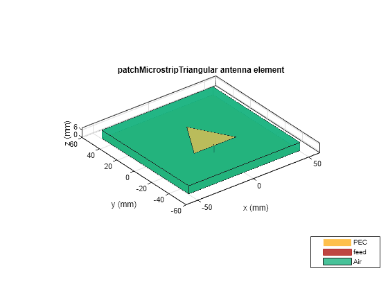
Create Triangular Patch Antenna
Create an equilateral triangular patch antenna with 37.63 mm patch sides. The feed is offset by 3.8 mm from the origin along the Y-axis.
side = 37.63e-3;
offset4 = 3.8e-3;
Use the patchMicrostripTriangular object to create this antenna using the defined parameters.
p_Triangular = patchMicrostripTriangular(Side=side,Height=thickness,Substrate=d,...
    GroundPlaneLength=lengthGp,GroundPlaneWidth=widthGp,...
    FeedOffset=[0 -side/2+offset4]);
[~] = mesh(p_Triangular,MaxEdgeLength=0.012)
figure
show(p_Triangular)
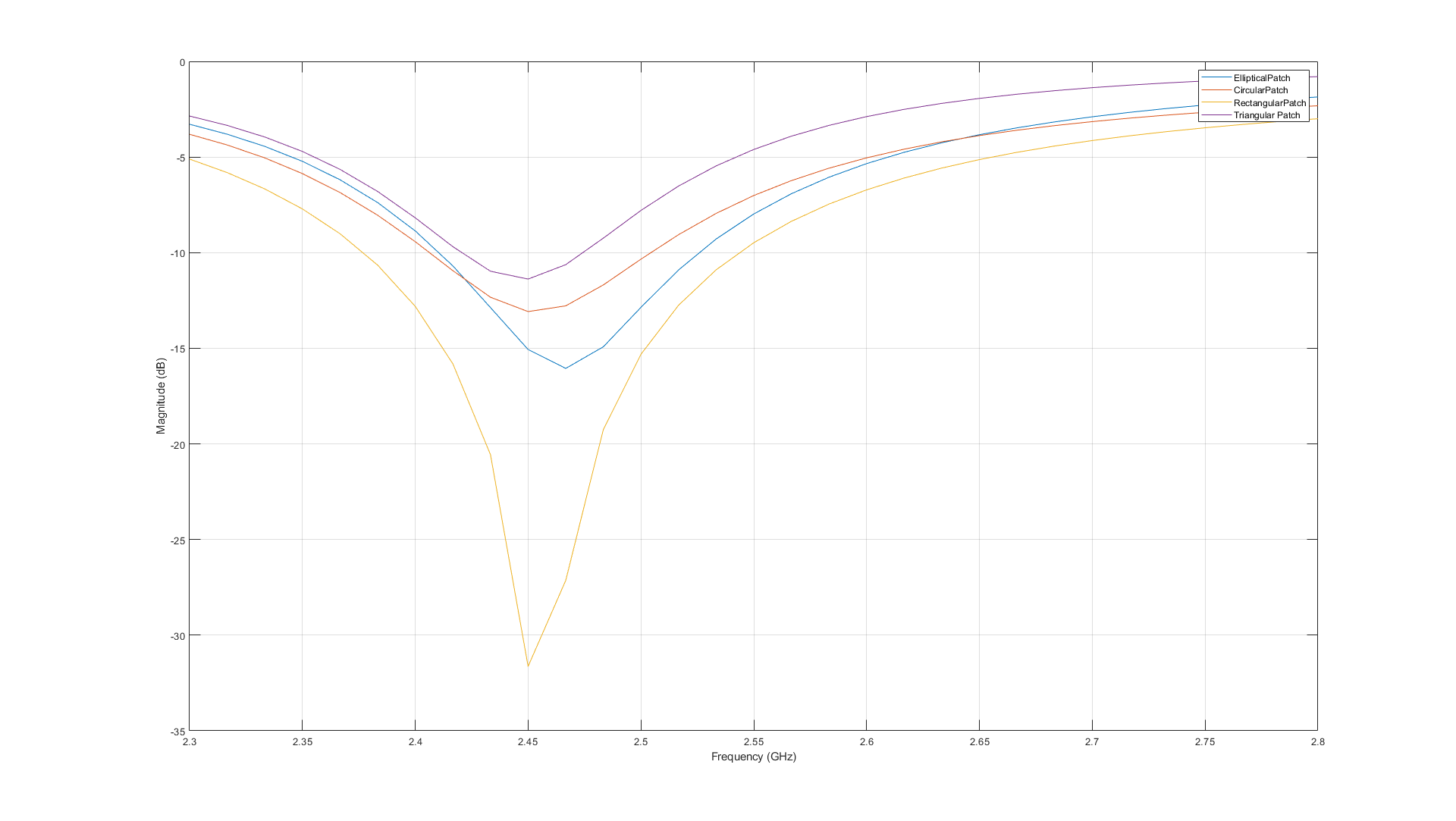
Visualize Reflection Coefficient Magnitude of Patch Antennas
Plot the reflection coefficient for these antennas over the 2.3 GHz - 2.8 GHz frequency range with a reference impedance of 50. A plot of the reflection coefficient magnitudes is shown in the following figure.
s1 = sparameters(p_Elliptical,freq);
s2 = sparameters(p_Circular,freq);
s3 = sparameters(p_Rectangular,freq);
s4 = sparameters(p_Triangular,freq);
figure
rfplot(s1);
hold on
rfplot(s2);
hold on
rfplot(s3);
hold on
rfplot(s4);
hold off
legend("dB(S_1_1) Elliptical Patch","dB(S_1_1) Circular Patch","dB(S_1_1) Rectangular Patch","dB(S_1_1) Triangular Patch",Location="southeast");
title("S-parameters")
Visualize Radiation Pattern of Patch Antennas
The directivities of these antennas are around:
6.37 dBi for the elliptical patch.
7 dBi for the circular patch.
7.37 dBi for the rectangular patch.
6.16 dBi for the triangular patch.
Visualize the directivities of these antennas.
dirElliptical = patternElevation(p_Elliptical,2.45e9);
dirCircular = patternElevation(p_Circular,2.45e9);
dirRectangular = patternElevation(p_Rectangular,2.45e9);
dirTriangular = patternElevation(p_Triangular,2.45e9);
figure
polarpattern(dirElliptical,TitleTop="Directivity (dBi)");
hold on
polarpattern(dirCircular);
hold on
polarpattern(dirRectangular);
hold on
polarpattern(dirTriangular);
hold off
legend("Elliptical Patch","Circular Patch","Rectangular Patch","Triangular Patch",Location="northeast");

Mutual Coupling Between Rectangular and Triangular Patches
This section is devoted to the study of a array configuration with lowest mutual coupling. An array of rectangular and triangular patches has the lowest mutual coupling. Create an array of these patches and visualize its radiation pattern to gauge the effect of mutual coupling. Place these patches side-by-side at center of the rectangular 160 mm-by-100 mm ground plane. Set the spacing between these patches to lambda/2. Use FR4 dielectric material for the substrate.
Create Patch Shape
Create a ground plane with the defined dimensions and centered at the origin.
spacing = 0.0612;
lengthGp1 = 160e-3;
widthGp1 = 100e-3;
groundPlane1 = antenna.Rectangle(Length=lengthGp1,Width=widthGp1);
Use pcbStack object to convert the rectangular patch antenna created previously to a PCB layer stack. Extract the patch shape from its metal layer. Position the shape so that its center lies at a distance spacing/2 from the center of the ground plane along the negative x-axis.
r_ant = pcbStack(p_Rectangular);
patchRectangular = r_ant.Layers{1};
patchRectangular.Center = [-spacing/2 0];
Use pcbStack object to convert the triangular patch antenna created previously to a PCB layer stack. Extract the patch shape from its metal layer. Position the shape so that its center lies at a distance spacing/2 from the center of the ground plane along the positive x-axis.
t_ant = pcbStack(p_Triangular);
patchTriangular = t_ant.Layers{1};
patchTriangular = rotateZ(patchTriangular,180);
patchTriangular = translate(patchTriangular,[spacing/2, 0, 0]);
Add these two shapes to get the final shape for the array.
patch = patchRectangular + patchTriangular;
Create Patch Antenna Array
Use the pcbStack object to define the metal and dielectric layers for mutually coupled patch antenna array. The top-most layer is a patch layer, the second layer is dielectric layer, and the third layer is the ground plane.
p_Coupled = pcbStack;
d4 = dielectric(EpsilonR=4.2,Thickness=thickness,LossTangent=0.02);
p_Coupled.BoardThickness = d4.Thickness;
p_Coupled.BoardShape.Length = lengthGp1;
p_Coupled.BoardShape.Width = widthGp1;
p_Coupled.Layers = {patch,d4,groundPlane1};
p_Coupled.FeedLocations = [-spacing/2 -(lengthRect/2-offset3) 1 3; spacing/2 -5.3075e-3 1 3];
p_Coupled.FeedDiameter = 1.3e-3;
figure
show(p_Coupled)
title("Patch Antenna Array");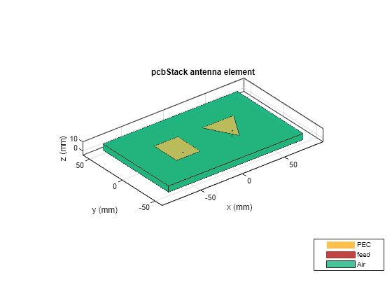
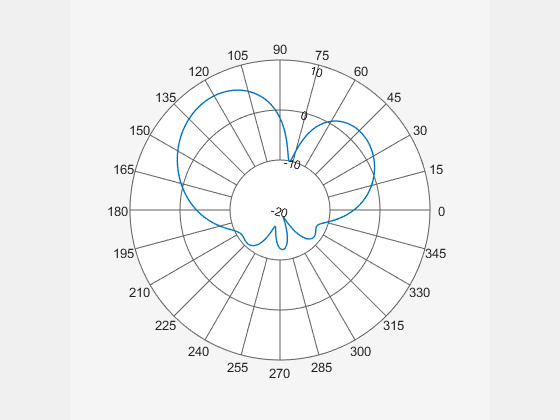
Radiation Pattern of Mutually Coupled Patch Antenna Array
Plot the directivity pattern of this patch antenna array at 2.45 GHz. The side-by-side patch configuration gives a directivity of around 7.64 dBi.
figure
pattern(p_Coupled,2.45e9,Type="directivity");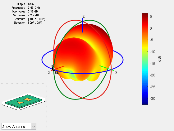
Warning: An error occurred while drawing the scene: GraphicsView error in command: interactionsmanagermessage:  TypeError: Cannot read properties of null (reading '_gview')
    at new g (https://127.0.0.1:31515/toolbox/matlab/uitools/figurelibjs/release/bundle.mwBundle.gbtfigure-lib.js?mre=https
Pattern Magnitude
Plot the elevation pattern of this patch antenna array.
figure
[mag,~,el] = pattern(p_Coupled,2.45e9,0,0:360,Type="directivity");
polarpattern(el,mag,TitleTop="Directivity in Elevation Plane (Azimuth=0)");
Reference
[1] Nascimento, D.C., and J.C. Da S. Lacava. “Design of Arrays of Linearly Polarized Patch Antennas on an FR4 Substrate: Design of a Probe-Fed Electrically Equivalent Microstrip Radiator.” IEEE Antennas and Propagation Magazine 57, no. 4 (August 2015): 12–22. https://doi.org/10.1109/MAP.2015.2453916.
See Also
Multiband Nature and Miniaturization of Fractal Antennas | Modeling and Analysis of Probe-Fed Stacked Patch Antenna