Planning Radar Network Coverage over Terrain

Import Terrain Data

Import DTED-format terrain data for a region around Boulder, Colorado, US. The terrain file was downloaded from the SRTM Void Filled data set available from the United States Geological Survey (USGS). The file is DTED level-1 format and has a sampling resolution of about 90 meters. A single DTED file defines a region that spans 1 degree in both latitude and longitude.

dtedfile = "n39_w106_3arc_v2.dt1";
attribution = "SRTM 3 arc-second resolution. Data available from the U.S. Geological Survey.";
addCustomTerrain("southboulder",dtedfile,"Attribution",attribution)

Open Site Viewer using the imported terrain. Visualization with high-resolution satellite map imagery requires an Internet connection.

viewer = siteviewer("Terrain","southboulder");

Show Candidate Radar Sites

The region contains mountains to the west and flatter areas to the east. Radars will be placed in the flat area to detect targets over the mountainous region. Define five candidate locations for placing the radars and show them on the map. The candidate locations are chosen to correspond to local high points on the map outside of residential areas.

Create collocated transmitter and receiver sites at each location to model monostatic radars, where the radar antennas are assumed to be 10 meters above ground level.

names = "Radar site" + (1:5);
rdrlats = [39.6055 39.6481 39.7015 39.7469 39.8856];
rdrlons = [-105.1602 -105.1378 -105.1772 -105.2000 -105.2181];

% Create transmitter sites associated with radars
rdrtxs = txsite("Name",names, ...
    "AntennaHeight",10, ...
    "Latitude",rdrlats, ...
    "Longitude",rdrlons);

% Create receiver sites associated with radars
rdrrxs = rxsite("Name",names, ...
    "AntennaHeight",10, ...
    "Latitude",rdrlats, ...
    "Longitude",rdrlons);

% Show just the radar transmitter sites
show(rdrtxs);

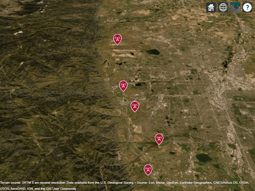
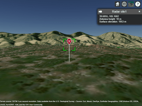
Zoom and rotate the map to view the 3-D terrain around the candidate radar sites. Select a site to view the location, antenna height, and ground elevation.

Design Monostatic Radar System

Design a basic monostatic pulse radar system to detect nonfluctuating targets with 0.1 square meter radar cross section (RCS) at a distance up to 35,000 meters from the radar with a range resolution of 5 meters. The desired performance index is a probability of detection (Pd) of 0.9 and probability of false alarm (Pfa) below 1e-6. The radars are assumed to be rotatable and support the same antenna gain in all directions, where the antenna gain corresponds to a highly directional antenna array.

pd = 0.9;         % Probability of detection
pfa = 1e-6;       % Probability of false alarm
maxrange = 35000; % Maximum unambiguous range (m)
rangeres = 5;     % Required range resolution (m)
tgtrcs = .1;      % Required target radar cross section (m^2)

Use pulse integration to reduce the required SNR at the radar receiver. Use 10 pulses and compute the SNR required to detect a target.

numpulses = 10;
snrthreshold = albersheim(pd, pfa, numpulses); % Unit: dB
disp(snrthreshold);

    4.9904

Define radar center frequency and antenna gain assuming a highly directional antenna array.

fc = 10e9;    % Transmitter frequency: 10 GHz
antgain = 38; % Antenna gain: 38 dB
c = physconst('LightSpeed');
lambda = c/fc;

Calculate the required peak pulse power (Watts) of the radar transmitter using the radar equation.

pulsebw = c/(2*rangeres);
pulsewidth = 1/pulsebw;
Ptx = radareqpow(lambda,maxrange,snrthreshold,pulsewidth,...
    'RCS',tgtrcs,'Gain',antgain);
disp(Ptx)

   3.1521e+05

Define Target Positions

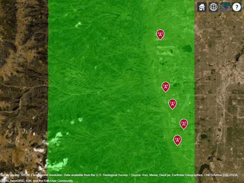
Define a grid containing 2500 locations to represent the geographic range of positions for a moving target in the region of interest. The region of interest spans 0.5 degrees in both latitude and longitude and includes mountains to the west as well as some of the area around the radar sites. The goal is to detect targets that are in the mountainous region to the west.

% Define region of interest
latlims = [39.5 40];
lonlims = [-105.6 -105.1];

% Define grid of target locations in region of interest
tgtlatv = linspace(latlims(1),latlims(2),50);
tgtlonv = linspace(lonlims(1),lonlims(2),50);
[tgtlons,tgtlats] = meshgrid(tgtlonv,tgtlatv);
tgtlons = tgtlons(:);
tgtlats = tgtlats(:);

Compute the minimum, maximum, and mean ground elevation for the target locations.

% Create temporary array of sites corresponding to target locations and query terrain
Z = elevation(txsite("Latitude",tgtlats,"Longitude",tgtlons));
[Zmin, Zmax] = bounds(Z);
Zmean = mean(Z);

disp("Ground elevation (meters): Min    Max    Mean" + newline + ...
    "                           " + round(Zmin) + "   " + round(Zmax) + "   " + round(Zmean))

Ground elevation (meters): Min    Max    Mean
                           1257   3953   2373

Target altitude can be defined with reference to mean sea level or to ground level. Use ground level as the reference and define a target altitude of 500 meters.

% Target altitude above ground level (m)
tgtalt = 500;

Show the region of interest as a solid green area on the map.

viewer.Name = "Radar Coverage Region of Interest";
regionData = propagationData(tgtlats,tgtlons,'Area',ones(size(tgtlats)));
contour(regionData,'ShowLegend',false,'Colors','green','Levels',0)

Calculate SNR for Target Positions with Terrain

The radar equation includes free space path loss and has a parameter for additional losses. Use a terrain propagation model to predict the additional path loss over terrain. Use TIREM™ from Huntington Ingalls Industries if it is available, or else use the Longley-Rice (ITM) model. TIREM™ supports frequencies up to 1000 GHz, whereas Longley-Rice is valid up to 20 GHz. Compute total additional loss including propagation from the radar to the target and then back from the target to the receiver.

% Create a terrain propagation model, using TIREM or Longley-Rice
tiremloc = tiremSetup;
if ~isempty(tiremloc)
    pm = propagationModel('tirem');
else
    pm = propagationModel('longley-rice');
end

% Compute additional path loss due to terrain and return distances between radars and targets 
[L, ds] = helperPathlossOverTerrain(pm, rdrtxs, rdrrxs, tgtlats, tgtlons, tgtalt);

Use the radar equation to compute the SNR at each radar receiver for the signal reflected from each target.

% Compute SNR for all radars and targets
numtgts = numel(tgtlats);
numrdrs = numel(rdrtxs);
rawsnr = zeros(numtgts,numrdrs);
for tgtind = 1:numtgts
    for rdrind = 1:numrdrs
        rawsnr(tgtind,rdrind) = radareqsnr(lambda,ds(tgtind,rdrind),Ptx,pulsewidth, ...
            'Gain',antgain,'RCS',tgtrcs,'Loss',L(tgtind,rdrind));
    end
end

Optimize Radar Coverage

A target is detected if the radar receiver SNR exceeds the SNR threshold computed above. Consider all combinations of radar sites and select the three sites that produce the highest number of detections. Compute the SNR data as the best SNR available at the receiver of any of the selected radar sites.

bestsitenums = helperOptimizeRadarSites(rawsnr, snrthreshold);
snr = max(rawsnr(:,bestsitenums),[],2);

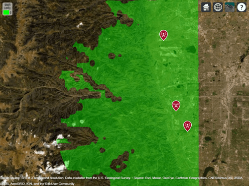
Display radar coverage showing the area where the SNR meets the required threshold to detect a target. The three radar sites selected for best coverage are shown using red markers.

The coverage map shows straight edges on the north, east, and south sides corresponding to the limits of the region of interest. The coverage map assumes that the radars can rotate and produce the same antenna gain in all directions and that the radars can transmit and receive simultaneously so that there is no minimum coverage range.

The coverage map has jagged portions on the western edge where the coverage areas are limited by terrain effects. A smooth portion of the western edge appears where the coverage is limited by the design range of the radar system, which is 35000 meters.

% Show selected radar sites using red markers
viewer.Name = "Radar Coverage";
clearMap(viewer)
show(rdrtxs(bestsitenums))

% Plot radar coverage
rdrData = propagationData(tgtlats,tgtlons,"SNR",snr);
legendTitle = "SNR" + newline + "(dB)";
contour(rdrData, ...
   "Levels",snrthreshold, ...
   "Colors","green", ...
   "LegendTitle",legendTitle)

Vary the Number of Pulses to Integrate

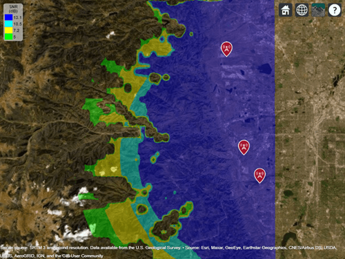
The previous analysis optimized radar transmitter power and site locations based on a system that integrates 10 pulses. Now investigate the impact on radar coverage for different modes of operation of the system, where the number of pulses to integrate is varied. Compute the SNR thresholds required to detect a target for varying number of pulses.

% Calculate SNR thresholds corresponding to different number of pulses
numpulses = 1:10;
snrthresholds = zeros(1,numel(numpulses));
for k = 1:numel(numpulses)
    snrthresholds(k) = albersheim(pd, pfa, numpulses(k));
end

% Plot SNR thresholds vs number of pulses to integrate
plot(numpulses,snrthresholds,'-*')
title("SNR at Radar Receiver Required for Detection")
xlabel("Number of pulses to integrate")
ylabel("SNR (dB)")
grid on;

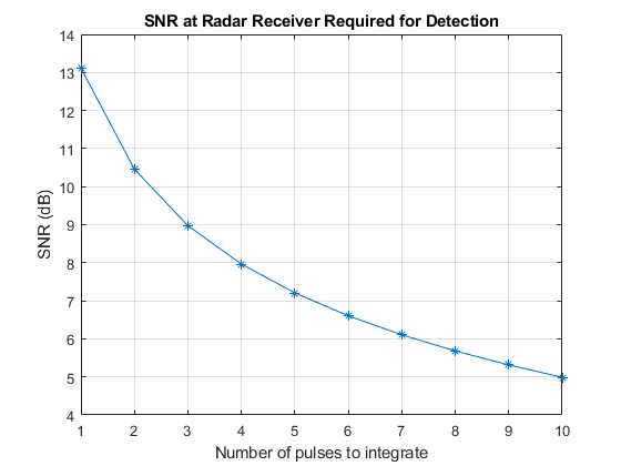
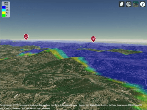
Show the radar coverage map for SNR thresholds corresponding to a few different numbers of pulses to integrate. Increasing the number of pulses to integrate decreases the required SNR and therefore produces a larger coverage region.

% Show best sites
viewer.Name = "Radar Coverage for Multiple SNR Thresholds";
show(rdrtxs(bestsitenums))

colors = jet(4);
colors(4,:) = [0 1 0];
contour(rdrData, ...
   "Levels",snrthresholds([1 2 5 10]), ...
   "Colors",colors, ...
   "LegendTitle",legendTitle)

Update Target Altitude

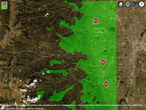
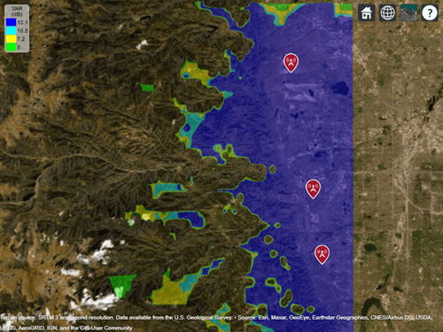
Update the scenario so that target positions are 250 meters above ground level instead of 500 meters above ground level. Rerun the same analysis as above to select the three best radar sites and visualize coverage. The new coverage map shows that reducing the visibility of the targets also decreases the coverage area.

% Target altitude above ground (m)
tgtalt = 250;
[L, ds] = helperPathlossOverTerrain(pm, rdrtxs, rdrrxs, tgtlats, tgtlons, tgtalt);

% Compute SNR for all radars and targets
numrdrs = numel(rdrtxs);
rawsnr = zeros(numtgts,numrdrs);
for tgtind = 1:numtgts
    for rdrind = 1:numrdrs
        rawsnr(tgtind,rdrind) = radareqsnr(lambda,ds(tgtind,rdrind),Ptx,pulsewidth, ...
            'Gain',antgain,'RCS',tgtrcs,'Loss',L(tgtind,rdrind));
    end
end

% Select best combination of 3 radar sites
bestsitenums = helperOptimizeRadarSites(rawsnr, snrthreshold);
snr = max(rawsnr(:,bestsitenums),[],2);

% Show best sites
viewer.Name = "Radar Coverage";
clearMap(viewer);
show(rdrtxs(bestsitenums))

% Plot radar coverage
rdrData = propagationData(tgtlats,tgtlons,"SNR",snr);
contour(rdrData, ...
   "Levels",snrthreshold, ...
   "Colors","green", ...
   "LegendTitle",legendTitle)

Show the radar coverage map for multiple SNR thresholds.

% Show best sites
viewer.Name = "Radar Coverage for Multiple SNR Thresholds";
show(rdrtxs(bestsitenums))

contour(rdrData, ...
   "Levels",snrthresholds([1 2 5 10]), ...
   "Colors",colors, ...
   "LegendTitle",legendTitle)

Conclusion

A monostatic radar system was designed to detect non-fluctuating targets with 0.1 square meter radar cross section (RCS) at a distance up to 35000 meters. Radar sites were selected among five candidate sites to optimize number of detections over a region of interest. Two target altitudes were considered: 500 meters above ground level and 250 meters above ground level. The coverage maps suggest the importance of line-of-sight visibility between the radar and target in order to achieve detection. The second scenario results in targets that are closer to ground level and therefore more likely to be blocked from line-of-sight visibility with a radar. This can be seen by rotating the map to view terrain, where non-coverage areas are typically located in shadow regions of the mountains.

Clean up by closing Site Viewer and removing the imported terrain data.

close(viewer)
removeCustomTerrain("southboulder")