Sensitivity Analysis for Antenna Using Monte-Carlo Simulation

Specify Design Variables

Set the design frequency to 3 GHz with corresponding free-space wavelength lambda. Choose these properties as design variables:

Set the initial values of the patch width and ground plane width as 0.25*lambda and 0.8*lambda, respectively. Limit the widths of the patch and the ground plane to within a range of 1.3 and 0.8 times of the initial values.

freq = 3e9;
lambda = 3e8/freq;
Np = 2;
pNames = {"GroundPlaneLength","Length"};
pInitVal = [0.8*lambda 0.25*lambda];
for m = 1:Np
    p(m,1) = param.Continuous(pNames{m},eye(1));
    p(m,1).Value = pInitVal(m);
p(m,1).Maximum = 1.3*pInitVal(m);
p(m,1).Minimum = 0.8*pInitVal(m);
end

Sample Design Space

Create a parameter space for the design variables using sdo.ParameterSpace (Simulink Design Optimization). The parameter space characterizes the allowable parameter values and combinations of parameter values.

pSpace = sdo.ParameterSpace(p);

The parameter space considers default uniform distributions for the design variables. Set lower and upper bounds of the distribution to the design variable minimum and maximum values, respectively. Use the sdo.sample (Simulink Design Optimization) function to generate samples from the parameter space. Use these samples to evaluate the model and explore the design space. Consider 10 sample points for the design space.

rng default;
nSamp=10;
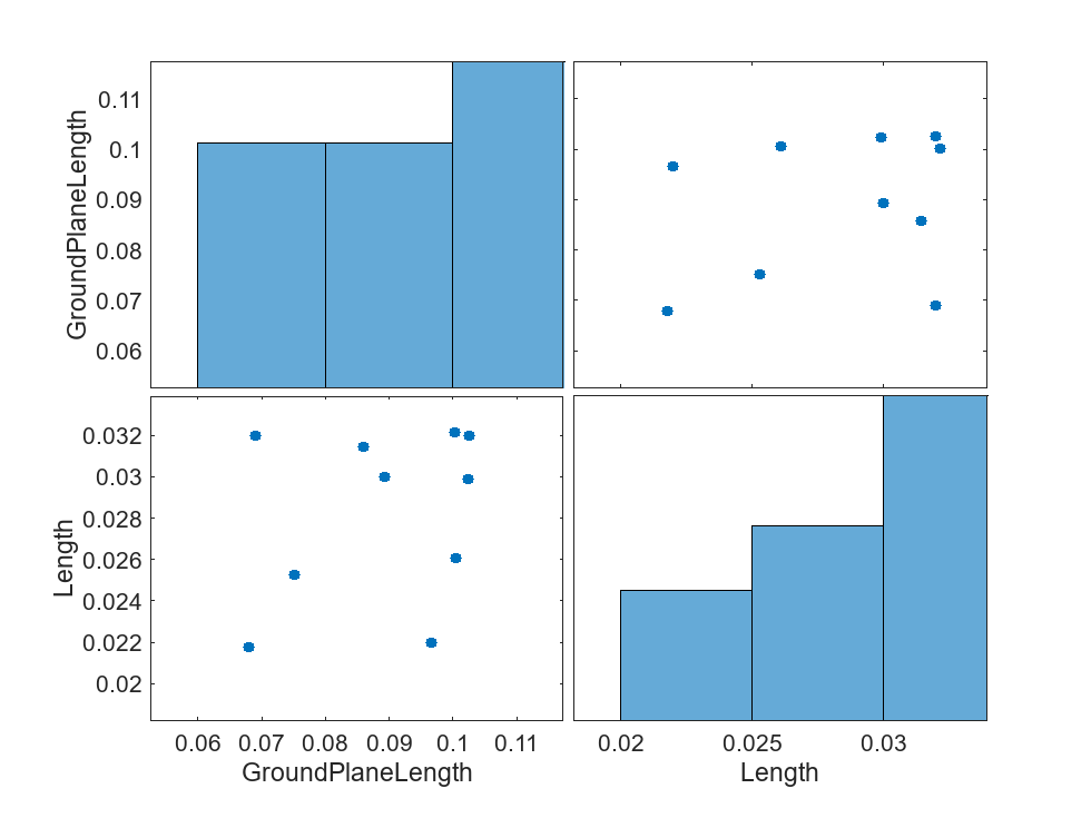
pSmpl = sdo.sample(pSpace,nSamp);

Use the sdo.scatterPlot (Simulink Design Optimization) function to visualize the sampled parameter space. The scatter plot shows parameter distributions on the diagonal subplots and pairwise parameter combinations on the off-diagonal subplots.

figure
sdo.scatterPlot(pSmpl)

Specify Uncertain Variables

Select the patch and ground plane lengths as uncertain variables. Evaluate the design using different patch and ground plane lengths. Set initial values of the patch and ground plane lengths to 0.25*lambda and 0.5*lambda, respectively. Limit the variation of these lengths to within 1.3 and 0.8 times the initial values.

npUnc = 2;
pUncNames = {"GroundPlaneWidth","Width"};
pUncInitVal = [0.5*lambda 0.25*lambda];
for m = 1:npUnc
    pUnc(m,1) = param.Continuous(pUncNames{m},eye(1));
    pUnc(m,1).Value = pUncInitVal(m);
pUnc(m,1).Maximum = 1.5*pUncInitVal(m);
pUnc(m,1).Minimum = 0.9*pUncInitVal(m);
end

Create a parameter space for the uncertain variables. Use normal distributions for both variables. Specify the mean as the current parameter value. Specify a variance of 5% of the mean for the GroundPlaneLength and 3% of the mean for the Length.

pUncDistributionType = {"normal","normal"};
pUncDistributionMean = [0.05 0.03];
uSpace = sdo.ParameterSpace(pUnc);
for m = 1:npUnc
    uSpace = setDistribution(uSpace,pUncNames{m},makedist(pUncDistributionType{m}, ...
        pUnc(m,1).Value,pUncDistributionMean(m)*pUnc(m,1).Value));
end

You can modify this information in the parameter space. This example considers an ideal correlation matrix.

uSpace.RankCorrelation = [1 0; 0 1];

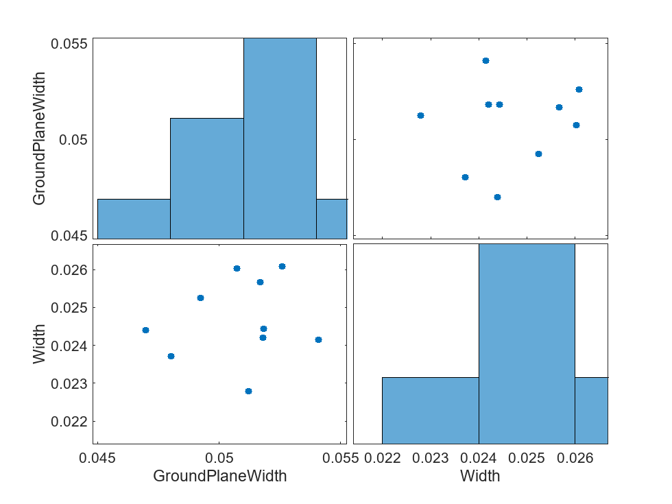
The rank correlation matrix has a row and column for each parameter. The entry in the ${\mathit{i}}^{\mathrm{th}}$ row and ${\mathit{j}}^{\mathrm{th}}$ column gives the correlation between parameters $\mathit{i}$ and $\mathit{j}$. Sample the parameter space. The scatter plot shows the correlation between the patch and ground plane length.

nSampUnc = 10;
uSmpl = sdo.sample(uSpace,nSampUnc);
figure
sdo.scatterPlot(uSmpl)

Ideally, you want to evaluate the design for every combination of points in the design and uncertain spaces, which implies (nSamp)*(nSampUnc) simulations. You can use parallel computing to speed up the evaluation.

Create Initial Antenna and Visualize the Geometry

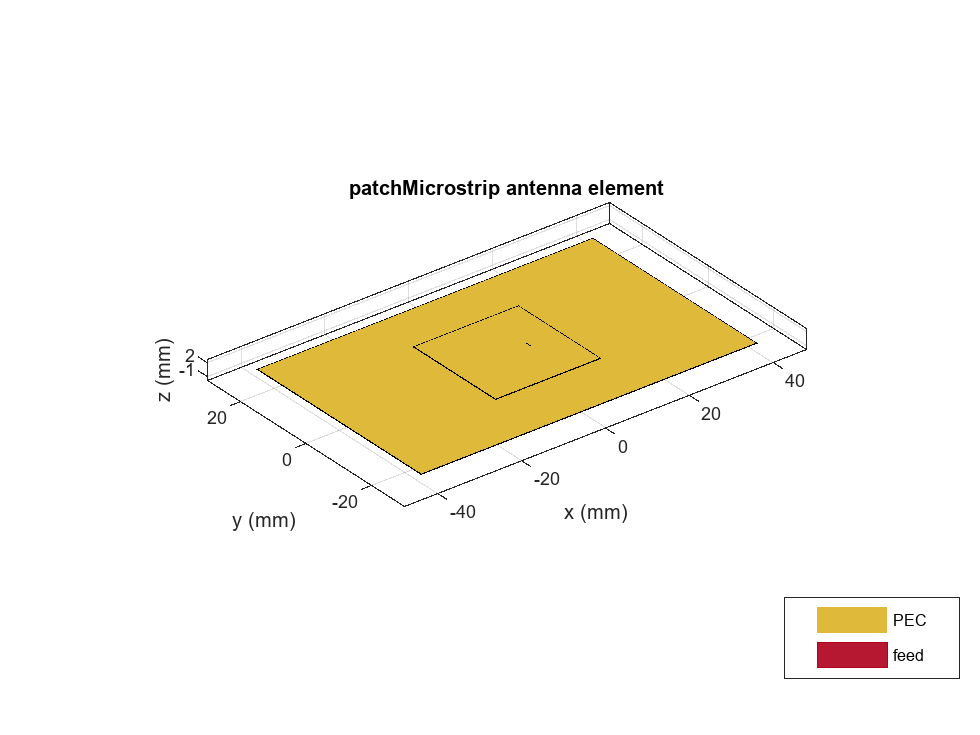
Create a microstrip patch antenna using the design function at 3 GHz. Set the patch and ground plane dimensions to their initial values and visualize the antenna.

ant = design(patchMicrostrip,freq);
ant.GroundPlaneLength = pInitVal(1);
ant.Length = pInitVal(2);
ant.GroundPlaneWidth = pUncInitVal(1);
ant.Width = pUncInitVal(2);
ant.Height = 0.8*1e-3;
ant.FeedOffset = [0.005 0];
figure
show(ant)

Specify Design Requirements

Evaluating a point in the design space requires specifying the expected threshold value. Here, you analyze the gain of the antenna. Compute the reference gain of the antenna using pattern with a logarithmic scale. Convert the gain value to a linear scale. Specify the number of iterations for the Monte-Carlo simulation. To reduce the simulation time, set the number of iterations to 10. Specify a higher value of numIterations for more accurate results.

gRef = max(max(pattern(ant,freq,Type="gain")));
linGain = 10^(0.1*gRef);
numIterations = 10;

Evaluate Antenna Design

Use iterative calls to construct the antenna for different property values and compute the gain. Check whether the computed gain meets the expected gain threshold to compute the cost function for the Monte-Carlo simulation.

probGain = zeros(size(pSmpl,1),1);
pSmpl_mat = table2array(pSmpl);
uSmpl_mat = table2array(uSmpl);
for i = 1:size(pSmpl_mat,1)   
     ant.GroundPlaneLength = pSmpl_mat(i,1);
     ant.Length = pSmpl_mat(i,2);  
     costGain = 0;
for index = 1:numIterations
for ct = 1:size(uSmpl_mat,1)      
    ant.GroundPlaneWidth = uSmpl_mat(ct,1);
    ant.Width = uSmpl_mat(ct,2);
    gainVal = max(max(pattern(ant,freq)));
    gainVal = 10^(0.1*gainVal);
    if gainVal>linGain
        costGain = costGain + 1;
    end    
end
end
probGain(i,1) = costGain/(numIterations*size(uSmpl_mat,1));
end

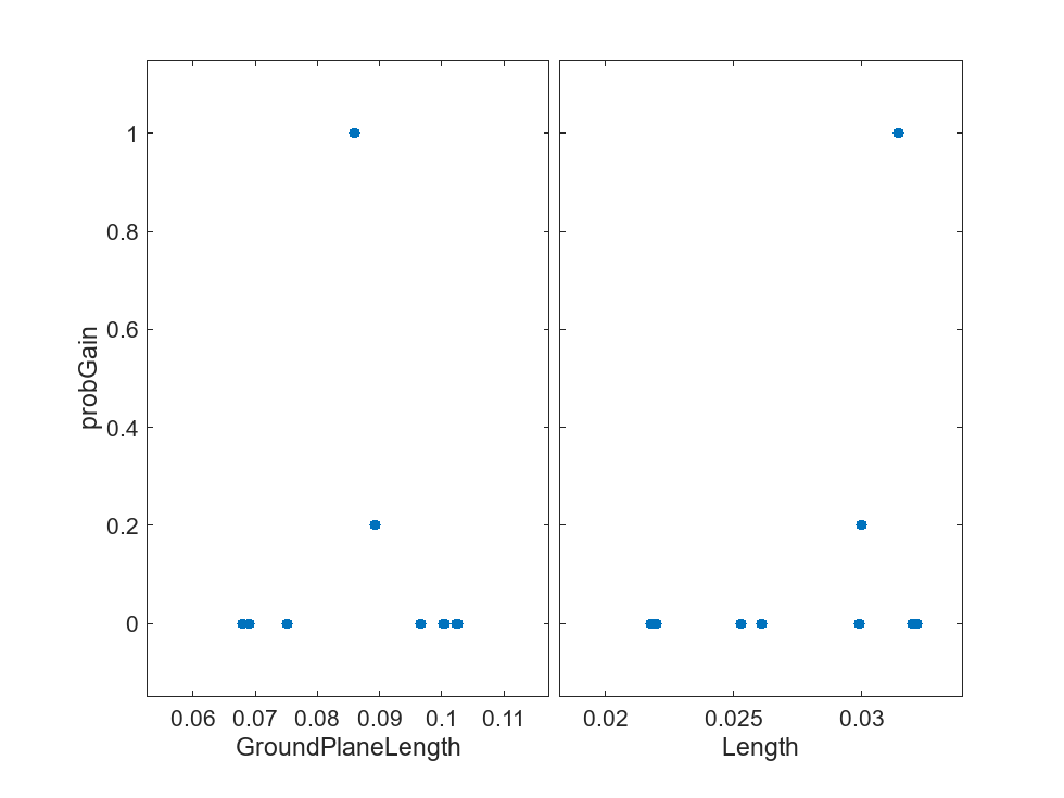
View the results of the evaluation using a scatter plot. The scatter plot shows pairwise plots for each design variable and design cost. The plot shows that larger cross-sectional areas result in lower total costs.

y = table(probGain);
figure
sdo.scatterPlot(pSmpl,y)

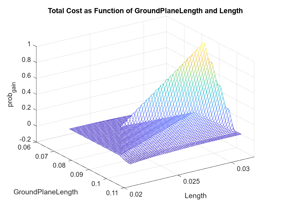
Create a mesh plot showing the total cost as a function of GroundPlaneLength and Length.

fTotal = scatteredInterpolant(pSmpl.GroundPlaneLength,...
    pSmpl.Length,y.probGain);
xR = linspace(min(pSmpl.GroundPlaneLength),max(pSmpl.GroundPlaneLength),60);
yR = linspace(min(pSmpl.Length),max(pSmpl.Length),60);
[xx,yy] = meshgrid(xR,yR);
zz = fTotal(xx,yy);
figure
mesh(xx,yy,zz)
view(56,30)
title("Total Cost as Function of GroundPlaneLength and Length")
zlabel("prob_{gain}");
xlabel(p(1).Name); 
ylabel(p(2).Name);

Further Exploration

You can further investigate the design variables of the antenna or array to perform sensitivity analysis on different output parameters like input impedance, gain, and efficiency. For an antenna or array configuration containing a large number of design variables, you can use this design space exploration approach to determine the most sensitive design parameters.