Design Series-Fed Patch Antenna Array for 5G Base Station

Create Variables

Create the variables and assign the values as per [2].

Wp = 3.539e-3;
Wc = 0.494e-3;
Lc = 3.539e-3;
Wm = 2.727e-3;
Lm = 0.6269e-3;
Wf = 0.72e-3;
Lf = 2.215e-3;

Create Geometry

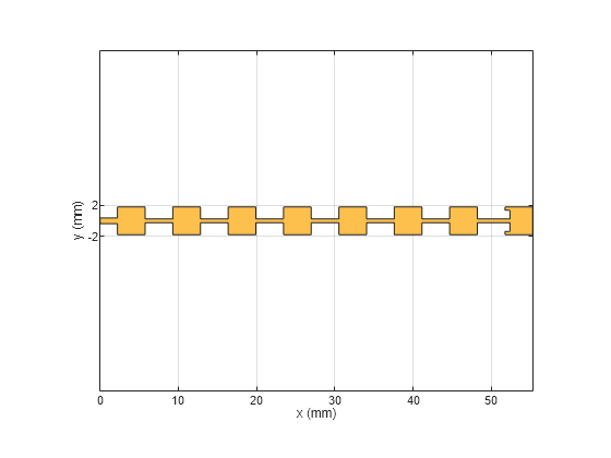
Use the antenna.Rectangle shape object to create all the rectangles in the structure and then join them. Visualize the structure using the show function.

a = antenna.Rectangle(Length=Lf,Width=Wf,Center=[Lf/2,0]);
transVec = Lf;
for i=1:7
b = antenna.Rectangle(Length=Wp,Width=Wp,Center=[transVec+Wp/2,0]);
transVec = transVec + Wp;
c = antenna.Rectangle(Length=Lc,Width=Wc,Center=[transVec+Lc/2,0]);
transVec = transVec + Lc;
a = a + b + c;
end
last = antenna.Rectangle(Length=Wp,Width=Wp,Center=[transVec+Wp/2,0]);
lastsub = antenna.Rectangle(Length=Lm,Width=Wm,Center=[transVec+Lm/2,0]);
last = last - lastsub;
conn = antenna.Rectangle(Length=Lc,Width=Wc,Center=[transVec+Lc/2,0]);
a = a + last + conn;
figure
show(a)

Design PCB Board

Use the pcbStack object to create the PCB stack. Create the ground plane and dielectric layers, and set the BoardShape to be the same shape as the ground plane. Visualize the PCB stack.

ant = pcbStack;
gnd = antenna.Rectangle(Length=57e-3,Width=10e-3,Center=[57e-3/2,0]);
d = dielectric("Teflon");
d.EpsilonR = 2.2;
ant.BoardThickness = 0.254e-3;
d.Thickness = ant.BoardThickness;
ant.Layers={a,d,gnd};
ant.BoardShape = gnd;
ant.FeedDiameter = Wf/2;
ant.FeedLocations = [0,0,1,3];
figure
show(ant)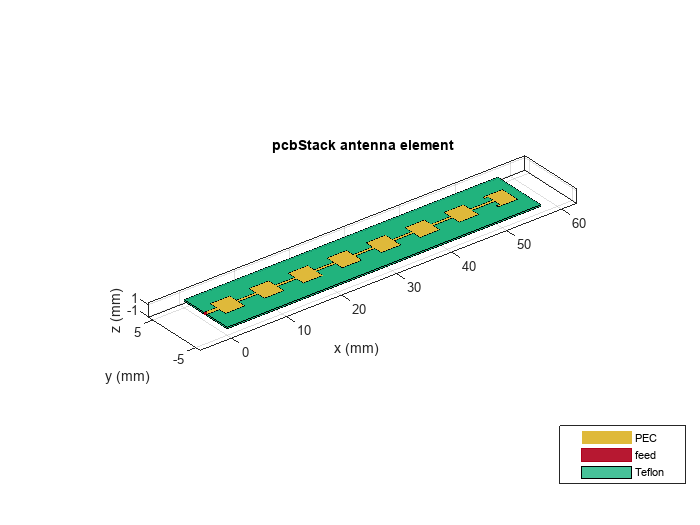

Analyze Array Performance

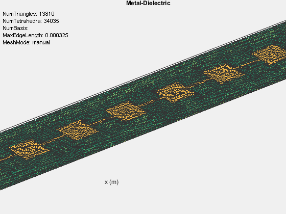
Use the mesh function to manually generate the mesh and set the MaxEdgeLength property to 0.4 mm to ensure there are 30 triangles per wavelength.

figure
mesh(ant,MaxEdgeLength=0.325e-3);
zoom(2.55)

Use the memoryEstimate function to calculate the memory required to solve the structure.

memEst = memoryEstimate(ant,28e9)

memEst = 
'43 GB'

As the memory requirement is very high, time required to calculate the S-parameters and plot the antenna pattern is quite high. This example includes a MAT file containing the return loss and pattern data computations. The code used to compute the results is available in the Return Loss and Pattern Data Computations section. On the machine with 64 GB of RAM and Intel(R) Xeon(R) W-2133 CPU processor it takes around 50 minutes to solve one frequency.

Load the MAT file and plot the return loss using the rfplot function.

load seriesPatchData.mat
figure
rfplot(out);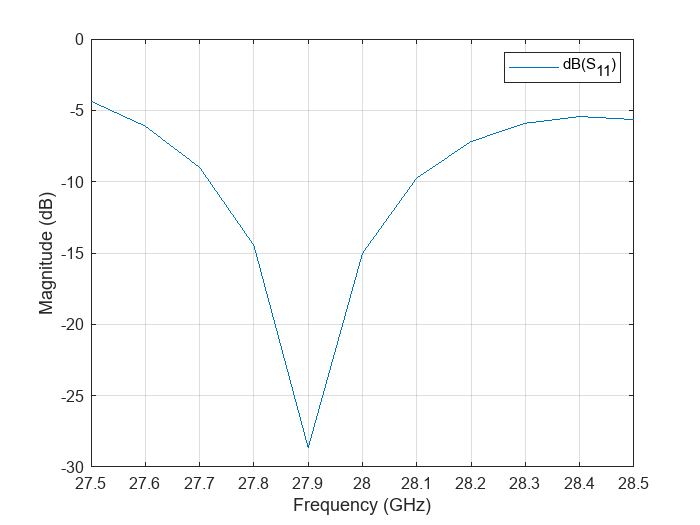

Use the patternCustom to plot the 2-D or 3-D radiation pattern of the antenna.

phi = az';
theta = (90-el);
MagE = pat';
figure
patternCustom(MagE,theta,phi);

Plot Radiation Pattern Using Pattern Multiplication

Use pattern multiplication to plot the radiation pattern of the 8-by-8 array instead of solving the entire structure using the MoM solver. You need a license to the Phased Array System Toolbox™ to use pattern multiplication.

Use the phased.CustomAntennaElement System object™ to build the custom antenna element using the pattern data from the loaded MAT file.

antenna = phased.CustomAntennaElement;
antenna.FrequencyVector = [0 28e9];
antenna.AzimuthAngles = az;
antenna.ElevationAngles = el;
antenna.MagnitudePattern = pat;
antenna.PhasePattern = zeros(size(pat));

Use the phased.ULA System object™ to create the 8-by-8 array. Specify the custom element as the array element. Set the number of elements to 8, and set the element spacing to 3.5 mm.

array = phased.ULA;
array.Element = antenna;
array.NumElements = 8;
array.ElementSpacing = 3.5e-3;

Pattern Multiplication

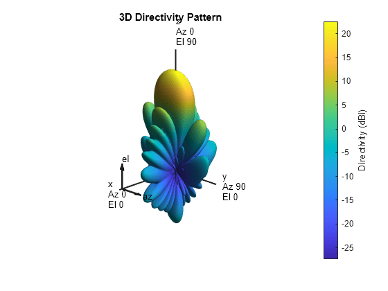
Use the pattern function to plot the 3-D radiation pattern.

figure
pattern(array,28e9)

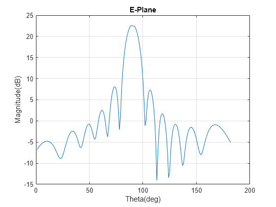
Use the pattern function to plot the radiation pattern in the E-plane.

pat1 = pattern(array,28e9,0,0:1:90,CoordinateSystem="rectangular");
pat2 = pattern(array,28e9,180,0:1:90,CoordinateSystem="rectangular");
data1 = [pat1; flip(pat2)];
figure
plot(data1);
grid on;
xlabel("Theta(deg)");
ylabel("Magnitude(dB)");
title("E-Plane");

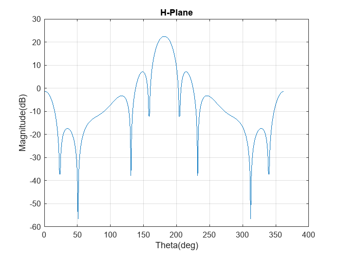
Use the pattern function to plot the radiation pattern in the H-plane.

pat3 = pattern(array,28e9,90,-90:1:90,CoordinateSystem="rectangular");
data2 = [pat3;flip(pat3)];
figure
plot(data2);
grid on;
xlabel("Theta(deg)");
ylabel("Magnitude(dB)");
title("H-Plane");

Return Loss and Pattern Data Computations

The following code was used to generate 'seriesPatchData.mat' file used in this example.

type RLpatDataComputation.m

out = sparameters(ant,linspace(27.5e9,28.5e9,11));
figure;
rfplot(out);
figure; 
pattern(ant, 28e9)
figure;
impedance(ant,linspace(27.5e9,28.5e9,11));

References

[1] “EM Simulation of 28 GHz Series-Fed Patch Antenna Array for 5G | 2019-02-01 | Microwave Journal.” Accessed January 21, 2022. https://www.microwavejournal.com/articles/31731-em-simulation-of-28-ghz-series-fed-patch-antenna-array-for-5g.

[2] Ishfaq, Muhammad Kamran, Tharek Abd Rahman, Yoshihide Yamada, and Kunio Sakakibara. “8×8 Phased Series Fed Patch Antenna Array at 28 GHz for 5G Mobile Base Station Antennas.” In 2017 IEEE-APS Topical Conference on Antennas and Propagation in Wireless Communications (APWC), 160–62. Verona, Italy: IEEE, 2017. https://doi.org/10.1109/APWC.2017.8062268.