Charge Distribution

The flow of charges on the antenna surface determines the surface currents of the antenna. For antennas to radiate, there must be acceleration or deceleration of charges. The deceleration of charges is caused due to buildup of charges at the end of the wire, which leads to impedance discontinuities. This mechanism creates electromagnetic radiation. The accumulation of charges varies according to time and structure of the antenna.

The accumulation of charges is exploited in many ways. If you calculate the impedance of this monopole antenna using the impedance function, you get the following plot:

m = monopole
impedance(m,20e6:1e6:120e6)

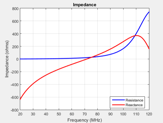
You can observe the first resonance is at approximately 71 MHz. To lower the resonance frequency, recalculate the height of the monopole to quarter wavelength. The frequency of operation is also lower. You must also have to increase the size of the corresponding ground plane. This increase in size means that to achieve similar performance at a lower frequency, you need a larger antenna. This approach is not possible due to physical space constraints.

Alternatively, you can exploit the fact that antennas have charge accumulation. If you provide appropriate structural modification to the antenna, charges accumulate. For a monopole antenna, you can enable charge accumulation by adding a top-hat to the monopole. Now, if you calculate the impedance of the antenna using the top-hat, the plot is:

mt = monopoleTopHat
impedance(mt,20e6:1e6:120e6)

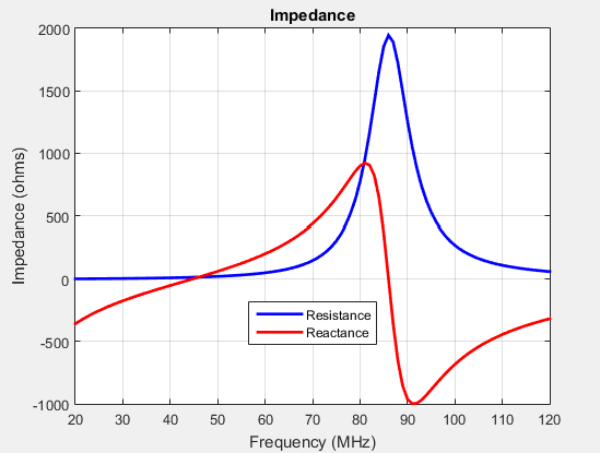
All the dimensions of this antenna are same as the monopole. The first resonance of the antenna is approximately 45 MHz. To view the accumulated charges on the top-hat monopole, use the charge function:

The increase in capacitance lowers the frequency of the antenna. By keeping the physical volume of the antenna same, the resonance point is shifted.

Increasing the top-hat dimensions provides more surface area for charges to accumulate. More charge accumulation increases the capacitance and pushes the resonant frequency lower. For example:

mt.TopHatLength = 0.35
mt.TopHatWidth = 0.35
impedance(mt,20e6:1e6:120e6)

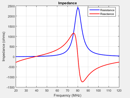
The resonance of the antenna further reduces to approximately 40 MHz.

Current Distribution

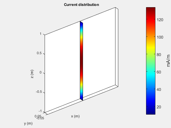
A typical antenna surface has current flowing on it. The behavior of the antenna surface current depends on the frequency of the input source, the geometry of the antenna, and the material properties of the antenna. The current is a vector and is spatially related to the structure of the antenna. In a dipole antenna, the maximum current distribution in the middle of the antenna and the minimum is toward the end:

d = dipole;
current(d,70e6)

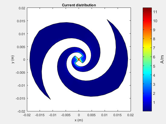
The same is true for a spiral antenna:

s = spiralEquiangular;
current(s,4e9)

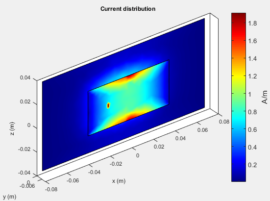
The patch also shows the current distribution of the classic $$\lambda /2$$ open-open resistor. The two ends of the patch represent an open circuit since the current is at a minimum.

pm = patchMicrostrip;
current(pm,1.75e9)

The spatial relationship between the current and structure of antenna is termed mode.

References

[1] Balanis, C.A. Antenna Theory. Analysis and Design, 3rd Ed. New York: Wiley, 2005.
[2] Makarov, S.N. Antenna and EM Modeling with MATLAB, New York: Wiley & Sons, 2002, p. 66.