Verification of Far-Field Array Pattern Using Superposition with Embedded Element Patterns

Set up Frequency and Array parameters

Choose the design frequency to be 1.8 GHz, which happens to be one of the carrier frequencies for 3G/4G cellular systems. Define array size using number of elements, N and inter-element spacing, dx.

fc = 1.8e9;
vp = physconst('lightspeed');
lambda0 = vp/fc;
N = 4;
dx = lambda0/2;

Design Antenna Element and Create the Array

For this example, we design a reflector backed half-wavelength dipole antenna. The reflector is half-wavelength in length along the x-axis and a quarter-wavelength in width, along the y-axis.

r = design(reflector,fc);
r.GroundPlaneLength = lambda0/2;
r.GroundPlaneWidth = lambda0/4;
figure
show(r)

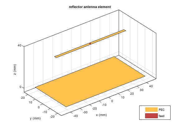
Use the reflector backed dipole as the individual element for the linear array. Use the NumElements property to change the linear array to have 4 elements instead of the default of 2. Change the element spacing to be half-wavelength.

lA = linearArray;
lA.Element = r;
lA.ElementSpacing = dx;
lA.NumElements = N;
figure
show(lA)

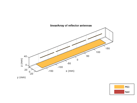
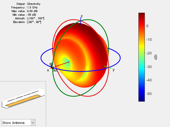
Calculate and Plot the 3D Array Pattern

By default all four elements in this array are excited with a voltage of 1V at a phase of 0 deg. Compute the far-field directivity pattern of this uniformly excited array at the center frequency.

figure
pattern(lA,fc)

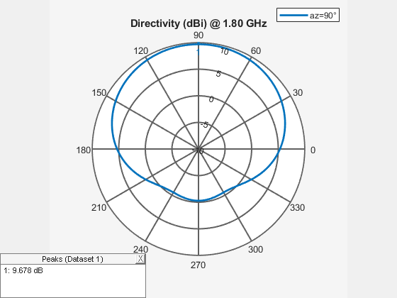
E and H-Plane Pattern Variation of the Fully Excited Array

The array being situated in the x-y plane results in most of the radiation being directed towards the zenith. The array pattern variations along the elevation angles can be captured along two orthogonal azimuth slices; at azimuth of 0° and at 90°. Visualize the directivity variation with elevation angle in these two planes is using the polarpattern function.

az = 0:5:360;
el = -180:1:180;

figure
patternElevation(lA,fc,0);

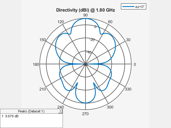
pE = polarpattern('gco');

figure
patternElevation(lA,fc,90);

pH = polarpattern('gco');

Calculate Embedded Element Complex Far-Fields

The embedded element pattern refers to the pattern of a single element embedded in the finite array, that is calculated by driving the central element in the array and terminating all other elements into a reference impedance [1]-[3]. The pattern of the driven element, referred to as the embedded element, incorporates the effect of coupling with the neighboring elements. In the Antenna Toolbox™, an ideal voltage source is used as excitation. To recreate the far-field pattern from superposition of the complex far-fields, use a very small value of resistance to terminate the remaining elements. Secondly, the superposition must be done on the complex far-field. Use the EHfields function to calculate the complex electric and magnetic fields at different points in space due to each excited element. For this example, choose a spherical arrangement of points in the E and H-plane angles defined earlier. The far-field points are computed at a radius of 100 $$\lambda$$.

R = 100*299792458/min(fc);
phi1 = az;
theta1 = 90-el;
[theta, phi] = meshgrid(theta1, phi1);  
phi = phi(:);
theta = theta(:);
X = R.*sind(theta).*cosd(phi);
Y = R.*sind(theta).*sind(phi);
Z = R.*cosd(theta);
Points = [X';Y';Z'];
N = lA.NumElements;
E = zeros(3,size(Points,2),N);
for i = 1:N
    E(:,:,i) = EHfields(lA,fc,Points,'ElementNumber',i,'Termination',1e-12);                                 
end

Superposition of Embedded Element Pattern Fields

Combine the individual embedded element electric field patterns in the far-field. For the sake of comparison with the pattern of the fully excited array, compute the magnitude. This will be used to calculate the total directivity in the E and H-plane respectively.

arrayEfieldpat = sum(E,3);
MagEsquare = dot(arrayEfieldpat, arrayEfieldpat);
MagE = sqrt(MagEsquare);
MagE = reshape(MagE,length(az),length(el));

Compute Directivity of Array

Directivity is a measure of the power projection ability of an antenna or array as a function of different angles in space. It defines the overall shape of the power projection capability of the radiating structure. To calculate this, find the radiation intensity in particular directions and divide it by the total radiated power from the structure over all directions. The total radiated power is computed as a product of the radiation efficiency and the input power. Each element of the array is assumed to be excited by a 1 Volt excitation source for computing the input power. The radiation efficiency of the array is computed using the efficiency function.

RadEff = efficiency(lA,fc);
InputPower = sum(0.5*real(1./conj(impedance(lA,fc))));
RadiatedPower = RadEff*InputPower;
eta = sqrt(1.25663706e-06/8.85418782e-12);
U = R^2*MagE.^2/(2*eta);
D = 10*log10(4*pi*U/RadiatedPower);

Comparison of Patterns

Overlay the directivity result from the superposition of the embedded element patterns on the result from the computation for the fully excited array.

idphi0  = find(az==0);
idphi90 = find(az==90);
Dphi    = D(idphi0,:);
Dphi90  = D(idphi90,:);
add(pE,el,Dphi);
pE.LegendLabels = {'Full-wave','Embedded superposition'};
pE.MagnitudeLim = [-40 20];
pE.Marker = {'+','.'};
pE.TitleTop = 'Elevation Slice @ az = 0 deg';

add(pH,el,Dphi90);
pH.LegendLabels = {'Full-wave','Embedded superposition'};
pH.MagnitudeLim = [-40 20];
pH.Marker = {'+','.'};
pH.TitleTop = 'Elevation Slice @ az = 90 deg';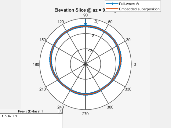

Summary

The use of superposition on the complex far-fields produced by the individual elements of an array generates the same pattern as the one from the uniformly excited array.

See Also

Modeling Mutual Coupling in Large Arrays Using Embedded Element Pattern

Reference

[1] R. J. Mailloux, 'Phased Array Antenna Handbook', Artech House, 2nd edition, 2005.

[2] W. Stutzman, G. Thiele, 'Antenna Theory and Design', John Wiley & Sons Inc., 3rd Edition, 2013.

[3] R. C. Hansen, Phased Array Antennas, Chapter 7 and 8, John Wiley & Sons Inc.,2nd Edition, 1998.