Cocktail Party Source Separation Using Deep Learning Networks

This example uses:

This example shows how to isolate a speech signal using a deep learning network.

Introduction

The cocktail party effect refers to the ability of the brain to focus on a single speaker while filtering out other voices and background noise. Humans perform very well at the cocktail party problem. This example shows how to use a deep learning network to separate individual speakers from a speech mix where one male and one female are speaking simultaneously.

Download Required Files

Before going into the example in detail, you will download a pre-trained network and 4 audio files.

downloadFolder = matlab.internal.examples.downloadSupportFile("audio/examples","cocktailpartyfc.zip");
dataFolder = tempdir;
dataset = fullfile(dataFolder,"CocktailPartySourceSeparation");
unzip(downloadFolder,dataset)

Problem Summary

Load audio files containing male and female speech sampled at 4 kHz. Listen to the audio files individually for reference.

[mSpeech,Fs] = audioread(fullfile(dataset,"MaleSpeech-16-4-mono-20secs.wav"));
sound(mSpeech,Fs)

[fSpeech] = audioread(fullfile(dataset,"FemaleSpeech-16-4-mono-20secs.wav"));
sound(fSpeech,Fs)

Combine the two speech sources. Ensure the sources have equal power in the mix. Scale the mix so that its max amplitude is one.

mSpeech = mSpeech/norm(mSpeech);
fSpeech = fSpeech/norm(fSpeech);

ampAdj = max(abs([mSpeech;fSpeech]));
mSpeech = mSpeech/ampAdj;
fSpeech = fSpeech/ampAdj;

mix = mSpeech + fSpeech;
mix = mix./max(abs(mix));

Visualize the original and mix signals. Listen to the mixed speech signal. This example shows a source separation scheme that extracts the male and female sources from the speech mix.

t = (0:numel(mix)-1)*(1/Fs);

figure
tiledlayout(3,1)

nexttile
plot(t,mSpeech)
title("Male Speech")
grid on

nexttile
plot(t,fSpeech)
title("Female Speech")
grid on

nexttile
plot(t,mix)
title("Speech Mix")
xlabel("Time (s)")
grid on

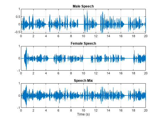
Figure contains 3 axes objects. Axes object 1 with title Male Speech contains an object of type line. Axes object 2 with title Female Speech contains an object of type line. Axes object 3 with title Speech Mix, xlabel Time (s) contains an object of type line.

Listen to the mix audio.

sound(mix,Fs)

Time-Frequency Representation

Use stft to visualize the time-frequency (TF) representation of the male, female, and mix speech signals. Use a Hann window of length 128, an FFT length of 128, and an overlap length of 96.

windowLength = 128;
fftLength = 128;
overlapLength = 96;
win = hann(windowLength,"periodic");

figure
tiledlayout(3,1)

nexttile
stft(mSpeech,Fs,Window=win,OverlapLength=overlapLength,FFTLength=fftLength,FrequencyRange="onesided");
title("Male Speech")

nexttile
stft(fSpeech,Fs,Window=win,OverlapLength=overlapLength,FFTLength=fftLength,FrequencyRange="onesided");
title("Female Speech")

nexttile
stft(mix,Fs,Window=win,OverlapLength=overlapLength,FFTLength=fftLength,FrequencyRange="onesided");
title("Mix Speech")

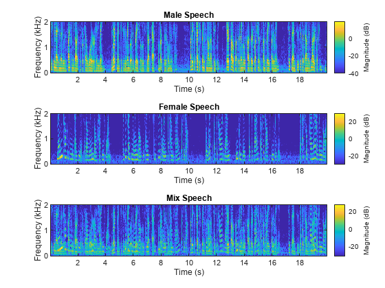
Figure contains 3 axes objects. Axes object 1 with title Male Speech, xlabel Time (s), ylabel Frequency (kHz) contains an object of type image. Axes object 2 with title Female Speech, xlabel Time (s), ylabel Frequency (kHz) contains an object of type image. Axes object 3 with title Mix Speech, xlabel Time (s), ylabel Frequency (kHz) contains an object of type image.

Source Separation Using Ideal Time-Frequency Masks

The application of a TF mask has been shown to be an effective method for separating desired audio signals from competing sounds. A TF mask is a matrix of the same size as the underlying STFT. The mask is multiplied element-by-element with the underlying STFT to isolate the desired source. The TF mask can be binary or soft.

Source Separation Using Ideal Binary Masks

In an ideal binary mask, the mask cell values are either 0 or 1. If the power of the desired source is greater than the combined power of other sources at a particular TF cell, then that cell is set to 1. Otherwise, the cell is set to 0.

Compute the ideal binary mask for the male speaker and then visualize it.

P_M = stft(mSpeech,Window=win,OverlapLength=overlapLength,FFTLength=fftLength,FrequencyRange="onesided");
P_F = stft(fSpeech,Window=win,OverlapLength=overlapLength,FFTLength=fftLength,FrequencyRange="onesided");
[P_mix,F] = stft(mix,Window=win,OverlapLength=overlapLength,FFTLength=fftLength,FrequencyRange="onesided");

binaryMask = abs(P_M) >= abs(P_F);

figure
plotMask(binaryMask,windowLength - overlapLength,F,Fs)

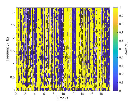
Figure contains an axes object. The axes object with xlabel Time (s), ylabel Frequency (Hz) contains an object of type image.

Estimate the male speech STFT by multiplying the mix STFT by the male speaker's binary mask. Estimate the female speech STFT by multiplying the mix STFT by the inverse of the male speaker's binary mask.

P_M_Hard = P_mix.*binaryMask;
P_F_Hard = P_mix.*(1-binaryMask);

Estimate the male and female audio signals using the inverse short-time FFT (ISTFT). Visualize the estimated and original signals. Listen to the estimated male and female speech signals.

mSpeech_Hard = istft(P_M_Hard,Window=win,OverlapLength=overlapLength,FFTLength=fftLength,FrequencyRange="onesided");
fSpeech_Hard = istft(P_F_Hard,Window=win,OverlapLength=overlapLength,FFTLength=fftLength,FrequencyRange="onesided");

figure
tiledlayout(2,2)

nexttile
plot(t,mSpeech)
axis([t(1) t(end) -1 1])
title("Original Male Speech")
grid on

nexttile
plot(t,mSpeech_Hard)
axis([t(1) t(end) -1 1])
xlabel("Time (s)")
title("Estimated Male Speech")
grid on

nexttile
plot(t,fSpeech)
axis([t(1) t(end) -1 1])
title("Original Female Speech")
grid on

nexttile
plot(t,fSpeech_Hard)
axis([t(1) t(end) -1 1])
title("Estimated Female Speech")
xlabel("Time (s)")
grid on

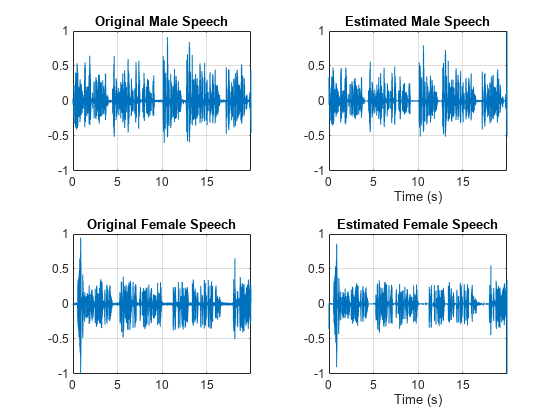
Figure contains 4 axes objects. Axes object 1 with title Original Male Speech contains an object of type line. Axes object 2 with title Estimated Male Speech, xlabel Time (s) contains an object of type line. Axes object 3 with title Original Female Speech contains an object of type line. Axes object 4 with title Estimated Female Speech, xlabel Time (s) contains an object of type line.

sound(mSpeech_Hard,Fs)

sound(fSpeech_Hard,Fs)

Source Separation Using Ideal Soft Masks

In a soft mask, the TF mask cell value is equal to the ratio of the desired source power to the total mix power. TF cells have values in the range [0,1].

Compute the soft mask for the male speaker. Estimate the STFT of the male speaker by multiplying the mix STFT by the male speaker's soft mask. Estimate the STFT of the female speaker by multiplying the mix STFT by the female speaker's soft mask.

Estimate the male and female audio signals using the ISTFT.

softMask = abs(P_M)./(abs(P_F) + abs(P_M) + eps);

P_M_Soft = P_mix.*softMask;
P_F_Soft = P_mix.*(1-softMask);

mSpeech_Soft = istft(P_M_Soft,Window=win,OverlapLength=overlapLength,FFTLength=fftLength,FrequencyRange="onesided");
fSpeech_Soft = istft(P_F_Soft,Window=win,OverlapLength=overlapLength,FFTLength=fftLength,FrequencyRange="onesided");

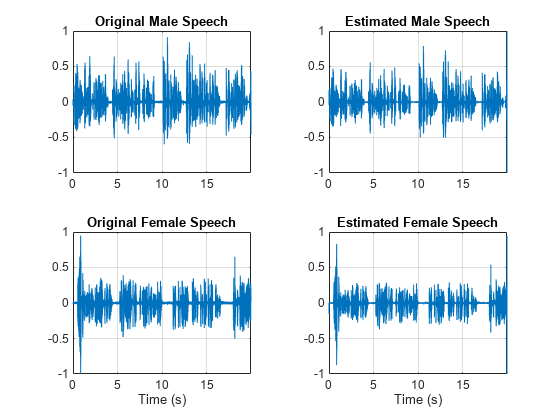
Visualize the estimated and original signals. Listen to the estimated male and female speech signals. Note that the results are very good because the mask is created with full knowledge of the separated male and female signals.

figure
tiledlayout(2,2)

nexttile
plot(t,mSpeech)
axis([t(1) t(end) -1 1])
title("Original Male Speech")
grid on

nexttile
plot(t,mSpeech_Soft)
axis([t(1) t(end) -1 1])
title("Estimated Male Speech")
grid on

nexttile
plot(t,fSpeech)
axis([t(1) t(end) -1 1])
xlabel("Time (s)")
title("Original Female Speech")
grid on

nexttile
plot(t,fSpeech_Soft)
axis([t(1) t(end) -1 1])
xlabel("Time (s)")
title("Estimated Female Speech")
grid on

Figure contains 4 axes objects. Axes object 1 with title Original Male Speech contains an object of type line. Axes object 2 with title Estimated Male Speech contains an object of type line. Axes object 3 with title Original Female Speech, xlabel Time (s) contains an object of type line. Axes object 4 with title Estimated Female Speech, xlabel Time (s) contains an object of type line.

sound(mSpeech_Soft,Fs)

sound(fSpeech_Soft,Fs)

Mask Estimation Using Deep Learning

The goal of the deep learning network in this example is to estimate the ideal soft mask described above. The network estimates the mask corresponding to the male speaker. The female speaker mask is derived directly from the male mask.

The basic deep learning training scheme is shown below. The predictor is the magnitude spectra of the mixed (male + female) audio. The target is the ideal soft masks corresponding to the male speaker. The regression network uses the predictor input to minimize the mean square error between its output and the input target. At the output, the audio STFT is converted back to the time domain using the output magnitude spectrum and the phase of the mix signal.

You transform the audio to the frequency domain using the Short-Time Fourier transform (STFT), with a window length of 128 samples, an overlap of 127, and a Hann window. You reduce the size of the spectral vector to 65 by dropping the frequency samples corresponding to negative frequencies (because the time-domain speech signal is real, this does not lead to any information loss). The predictor input consists of 20 consecutive STFT vectors. The output is a 65-by-20 soft mask.

You use the trained network to estimate the male speech. The input to the trained network is the mixture (male + female) speech audio.

STFT Targets and Predictors

This section illustrates how to generate the target and predictor signals from the training dataset.

Read in training signals consisting of around 400 seconds of speech from male and female speakers, respectively, sampled at 4 kHz. The low sample rate is used to speed up training. Trim the training signals so that they are the same length.

mSpeechTrain = audioread(fullfile(dataset,"MaleSpeech-16-4-mono-405secs.wav"));
fSpeechTrain = audioread(fullfile(dataset,"FemaleSpeech-16-4-mono-405secs.wav"));

L = min(length(mSpeechTrain),length(fSpeechTrain));  
mSpeechTrain = mSpeechTrain(1:L);
fSpeechTrain = fSpeechTrain(1:L);

Read in validation signals consisting of around 20 seconds of speech from male and female speakers, respectively, sampled at 4 kHz. Trim the validation signals so that they are the same length.

mSpeechValidate = audioread(fullfile(dataset,"MaleSpeech-16-4-mono-20secs.wav"));
fSpeechValidate = audioread(fullfile(dataset,"FemaleSpeech-16-4-mono-20secs.wav"));

L = min(length(mSpeechValidate),length(fSpeechValidate));  
mSpeechValidate = mSpeechValidate(1:L);
fSpeechValidate = fSpeechValidate(1:L);

Scale the training signals to the same power. Scale the validation signals to the same power.

mSpeechTrain = mSpeechTrain/norm(mSpeechTrain);
fSpeechTrain = fSpeechTrain/norm(fSpeechTrain);
ampAdj = max(abs([mSpeechTrain;fSpeechTrain]));

mSpeechTrain = mSpeechTrain/ampAdj;
fSpeechTrain = fSpeechTrain/ampAdj;

mSpeechValidate = mSpeechValidate/norm(mSpeechValidate);
fSpeechValidate = fSpeechValidate/norm(fSpeechValidate);
ampAdj = max(abs([mSpeechValidate;fSpeechValidate]));

mSpeechValidate = mSpeechValidate/ampAdj;
fSpeechValidate = fSpeechValidate/ampAdj;

Create the training and validation "cocktail party" mixes.

mixTrain = mSpeechTrain + fSpeechTrain;
mixTrain = mixTrain/max(mixTrain);

mixValidate = mSpeechValidate + fSpeechValidate;
mixValidate = mixValidate/max(mixValidate);

Generate training STFTs.

windowLength = 128;
fftLength = 128;
overlapLength = 128-1;
Fs = 4000;
win = hann(windowLength,"periodic");

P_mix0 = abs(stft(mixTrain,Window=win,OverlapLength=overlapLength,FFTLength=fftLength,FrequencyRange="onesided"));
P_M = abs(stft(mSpeechTrain,Window=win,OverlapLength=overlapLength,FFTLength=fftLength,FrequencyRange="onesided"));
P_F = abs(stft(fSpeechTrain,Window=win,OverlapLength=overlapLength,FFTLength=fftLength,FrequencyRange="onesided"));

Take the log of the mix STFT. Normalize the values by their mean and standard deviation.

P_mix = log(P_mix0 + eps);
MP = mean(P_mix(:));
SP = std(P_mix(:));
P_mix = (P_mix - MP)/SP;

Generate validation STFTs. Take the log of the mix STFT. Normalize the values by their mean and standard deviation.

P_Val_mix0 = stft(mixValidate,Window=win,OverlapLength=overlapLength,FFTLength=fftLength,FrequencyRange="onesided");
P_Val_M = abs(stft(mSpeechValidate,Window=win,OverlapLength=overlapLength,FFTLength=fftLength,FrequencyRange="onesided"));
P_Val_F = abs(stft(fSpeechValidate,Window=win,OverlapLength=overlapLength,FFTLength=fftLength,FrequencyRange="onesided"));

P_Val_mix = log(abs(P_Val_mix0) + eps);
MP = mean(P_Val_mix(:));
SP = std(P_Val_mix(:));
P_Val_mix = (P_Val_mix - MP) / SP;

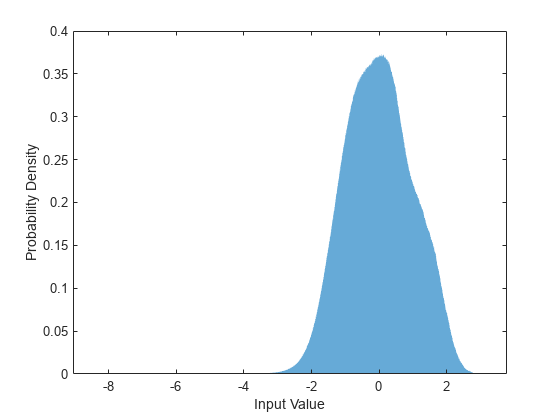
Training neural networks is easiest when the inputs to the network have a reasonably smooth distribution and are normalized. To check that the data distribution is smooth, plot a histogram of the STFT values of the training data.

figure
histogram(P_mix,EdgeColor="none",Normalization="pdf")
xlabel("Input Value")
ylabel("Probability Density")

Figure contains an axes object. The axes object with xlabel Input Value, ylabel Probability Density contains an object of type histogram.

Compute the training soft mask. Use this mask as the target signal while training the network.

maskTrain = P_M./(P_M + P_F + eps);

Compute the validation soft mask. Use this mask to evaluate the mask emitted by the trained network.

maskValidate = P_Val_M./(P_Val_M + P_Val_F + eps);

To check that the target data distribution is smooth, plot a histogram of the mask values of the training data.

figure

histogram(maskTrain,EdgeColor="none",Normalization="pdf")
xlabel("Input Value")
ylabel("Probability Density")

Figure contains an axes object. The axes object with xlabel Input Value, ylabel Probability Density contains an object of type histogram.

Create chunks of size (65, 20) from the predictor and target signals. In order to get more training samples, use an overlap of 10 segments between consecutive chunks.

seqLen = 20;
seqOverlap = 10;
mixSequences = zeros(1 + fftLength/2,seqLen,1,0);
maskSequences = zeros(1 + fftLength/2,seqLen,1,0);

loc = 1;
while loc < size(P_mix,2) - seqLen
    mixSequences(:,:,:,end+1) = P_mix(:,loc:loc+seqLen-1);
    maskSequences(:,:,:,end+1) = maskTrain(:,loc:loc+seqLen-1);
    loc = loc + seqOverlap;
end

Create chunks of size (65,20) from the validation predictor and target signals.

mixValSequences = zeros(1 + fftLength/2,seqLen,1,0);
maskValSequences = zeros(1 + fftLength/2,seqLen,1,0);
seqOverlap = seqLen;

loc = 1;
while loc < size(P_Val_mix,2) - seqLen
    mixValSequences(:,:,:,end+1) = P_Val_mix(:,loc:loc+seqLen-1);
    maskValSequences(:,:,:,end+1) = maskValidate(:,loc:loc+seqLen-1);
    loc = loc + seqOverlap;
end

Reshape the training and validation signals.

mixSequencesT = reshape(mixSequences,[1 1 (1 + fftLength/2)*seqLen size(mixSequences,4)]);
mixSequencesV = reshape(mixValSequences,[1 1 (1 + fftLength/2)*seqLen size(mixValSequences,4)]);
maskSequencesT = reshape(maskSequences,[1 1 (1 + fftLength/2)*seqLen size(maskSequences,4)]);
maskSequencesV = reshape(maskValSequences,[1 1 (1 + fftLength/2)*seqLen size(maskValSequences,4)]);

Define Deep Learning Network

Define the layers of the network. Specify the input size to be images of size 1-by-1-by-1300. Define two hidden fully connected layers, each with 1300 neurons. Follow each hidden fully connected layer with a biased sigmoid layer. The batch normalization layers normalize the means and standard deviations of the outputs. Add a fully connected layer with 1300 neurons.

numNodes = (1 + fftLength/2)*seqLen;

layers = [ ...
    
    imageInputLayer([1 1 (1 + fftLength/2)*seqLen],Normalization="None")
    
    fullyConnectedLayer(numNodes)
    BiasedSigmoidLayer(6)
    batchNormalizationLayer
    dropoutLayer(0.1)

    fullyConnectedLayer(numNodes)
    BiasedSigmoidLayer(6)
    batchNormalizationLayer
    dropoutLayer(0.1)

    fullyConnectedLayer(numNodes)
    BiasedSigmoidLayer(0)
    
    ];

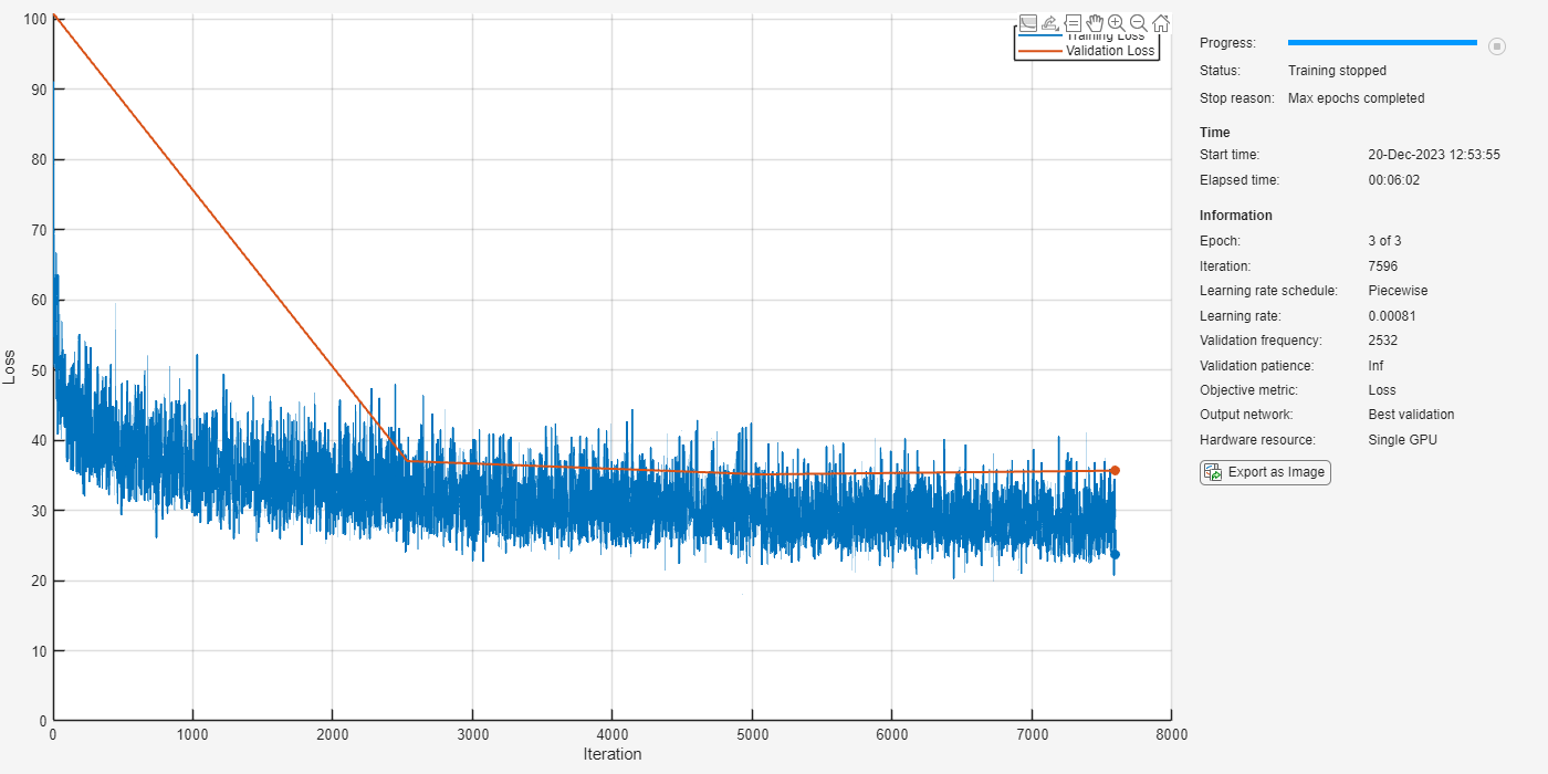
Specify the training options for the network. Set MaxEpochs to 3 so that the network makes three passes through the training data. Set MiniBatchSize to 64 so that the network looks at 64 training signals at a time. Set Plots to training-progress to generate plots that show the training progress as the number of iterations increases. Set Verbose to false to disable printing the table output that corresponds to the data shown in the plot into the command line window. Set Shuffle to every-epoch to shuffle the training sequences at the beginning of each epoch. Set LearnRateSchedule to piecewise to decrease the learning rate by a specified factor (0.1) every time a certain number of epochs (1) has passed. Set ValidationData to the validation predictors and targets. Set ValidationFrequency such that the validation mean square error is computed once per epoch. This example uses the adaptive moment estimation (ADAM) solver.

maxEpochs = 3;
miniBatchSize = 64;

options = trainingOptions("adam", ...
    MaxEpochs=maxEpochs, ...
    MiniBatchSize=miniBatchSize, ...
    SequenceLength="longest", ...
    Shuffle="every-epoch", ...
    Verbose=0, ...
    Plots="training-progress", ...
    ValidationFrequency=floor(size(mixSequencesT,4)/miniBatchSize), ...
    ValidationData={mixSequencesV,permute(maskSequencesV,[4 3 1 2])}, ...
    LearnRateSchedule="piecewise", ...
    LearnRateDropFactor=0.9, ...
    LearnRateDropPeriod=1);

Train Deep Learning Network

Train the network with the specified training options and layer architecture using trainnet. Because the training set is large, the training process can take several minutes. To load a pre-trained network, set speedupExample to true.

speedupExample = false;
if ~speedupExample
    lossFcn = @(Y,T)0.5*l2loss(Y,T,NormalizationFactor="batch-size");
    CocktailPartyNet = trainnet(mixSequencesT,permute(maskSequencesT,[4 3 1 2]),layers,lossFcn,options);
else
    s = load(fullfile(dataset,"CocktailPartyNet.mat"));
    CocktailPartyNet = s.CocktailPartyNet;
end

Pass the validation predictors to the network. The output is the estimated mask. Reshape the estimated mask.

estimatedMasks0 = predict(CocktailPartyNet,mixSequencesV);

estimatedMasks0 = estimatedMasks0.';
estimatedMasks0 = reshape(estimatedMasks0,1 + fftLength/2,numel(estimatedMasks0)/(1 + fftLength/2));

Evaluate Deep Learning Network

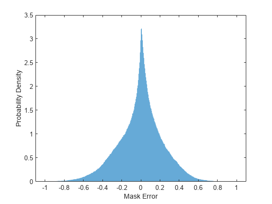
Plot a histogram of the error between the actual and expected mask.

figure
histogram(maskValSequences(:) - estimatedMasks0(:),EdgeColor="none",Normalization="pdf")
xlabel("Mask Error")
ylabel("Probability Density")

Figure contains an axes object. The axes object with xlabel Mask Error, ylabel Probability Density contains an object of type histogram.

Evaluate Soft Mask Estimation

Estimate male and female soft masks. Estimate male and female binary masks by thresholding the soft masks.

SoftMaleMask = estimatedMasks0; 
SoftFemaleMask = 1 - SoftMaleMask;

Shorten the mix STFT to match the size of the estimated mask.

P_Val_mix0 = P_Val_mix0(:,1:size(SoftMaleMask,2));

Multiply the mix STFT by the male soft mask to get the estimated male speech STFT.

P_Male = P_Val_mix0.*SoftMaleMask;

Use the ISTFT to get the estimated male audio signal. Scale the audio.

maleSpeech_est_soft = istft(P_Male,Window=win,OverlapLength=overlapLength,FFTLength=fftLength,FrequencyRange="onesided",ConjugateSymmetric=true);
maleSpeech_est_soft = maleSpeech_est_soft/max(abs(maleSpeech_est_soft));

Determine a range to analyze and the associated time vector.

range = windowLength:numel(maleSpeech_est_soft)-windowLength;
t = range*(1/Fs);

Visualize the estimated and original male speech signals. Listen to the estimated soft mask male speech.

sound(maleSpeech_est_soft(range),Fs)

figure
tiledlayout(2,1)

nexttile
plot(t,mSpeechValidate(range))
title("Original Male Speech")
xlabel("Time (s)")
grid on

nexttile
plot(t,maleSpeech_est_soft(range))
xlabel("Time (s)")
title("Estimated Male Speech (Soft Mask)")
grid on

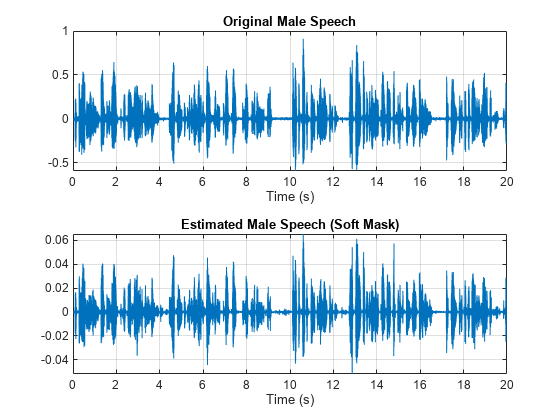
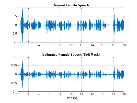
Figure contains 2 axes objects. Axes object 1 with title Original Male Speech, xlabel Time (s) contains an object of type line. Axes object 2 with title Estimated Male Speech (Soft Mask), xlabel Time (s) contains an object of type line.

Multiply the mix STFT by the female soft mask to get the estimated female speech STFT. Use the ISTFT to get the estimated male audio signal. Scale the audio.

P_Female = P_Val_mix0.*SoftFemaleMask;

femaleSpeech_est_soft = istft(P_Female,Window=win,OverlapLength=overlapLength,FFTLength=fftLength,FrequencyRange="onesided",ConjugateSymmetric=true);
femaleSpeech_est_soft = femaleSpeech_est_soft/max(femaleSpeech_est_soft);

Visualize the estimated and original female signals. Listen to the estimated female speech.

sound(femaleSpeech_est_soft(range),Fs)

figure
tiledlayout(2,1)

nexttile
plot(t,fSpeechValidate(range))
title("Original Female Speech")
grid on

nexttile
plot(t,femaleSpeech_est_soft(range))
xlabel("Time (s)")
title("Estimated Female Speech (Soft Mask)")
grid on

Figure contains 2 axes objects. Axes object 1 with title Original Female Speech contains an object of type line. Axes object 2 with title Estimated Female Speech (Soft Mask), xlabel Time (s) contains an object of type line.

Evaluate Binary Mask Estimation

Estimate male and female binary masks by thresholding the soft masks.

HardMaleMask = SoftMaleMask >= 0.5;
HardFemaleMask = SoftMaleMask < 0.5;

Multiply the mix STFT by the male binary mask to get the estimated male speech STFT. Use the ISTFT to get the estimated male audio signal. Scale the audio.

P_Male = P_Val_mix0.*HardMaleMask;

maleSpeech_est_hard = istft(P_Male,Window=win,OverlapLength=overlapLength,FFTLength=fftLength,FrequencyRange="onesided",ConjugateSymmetric=true);
maleSpeech_est_hard = maleSpeech_est_hard/max(maleSpeech_est_hard);

Visualize the estimated and original male speech signals. Listen to the estimated binary mask male speech.

sound(maleSpeech_est_hard(range),Fs)

figure
tiledlayout(2,1)

nexttile
plot(t,mSpeechValidate(range))
title("Original Male Speech")
grid on

nexttile
plot(t,maleSpeech_est_hard(range))
xlabel("Time (s)")
title("Estimated Male Speech (Binary Mask)")
grid on

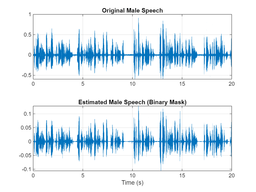
Figure contains 2 axes objects. Axes object 1 with title Original Male Speech contains an object of type line. Axes object 2 with title Estimated Male Speech (Binary Mask), xlabel Time (s) contains an object of type line.

Multiply the mix STFT by the female binary mask to get the estimated male speech STFT. Use the ISTFT to get the estimated male audio signal. Scale the audio.

P_Female = P_Val_mix0.*HardFemaleMask;

femaleSpeech_est_hard = istft(P_Female,Window=win,OverlapLength=overlapLength,FFTLength=fftLength,FrequencyRange="onesided",ConjugateSymmetric=true);
femaleSpeech_est_hard = femaleSpeech_est_hard/max(femaleSpeech_est_hard);

Visualize the estimated and original female speech signals. Listen to the estimated female speech.

sound(femaleSpeech_est_hard(range),Fs)

figure
tiledlayout(2,1)

nexttile
plot(t,fSpeechValidate(range))
title("Original Female Speech")
grid on

nexttile
plot(t,femaleSpeech_est_hard(range))
title("Estimated Female Speech (Binary Mask)")
grid on

Figure contains 2 axes objects. Axes object 1 with title Original Female Speech contains an object of type line. Axes object 2 with title Estimated Female Speech (Binary Mask) contains an object of type line.

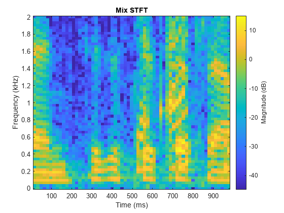
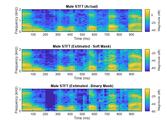
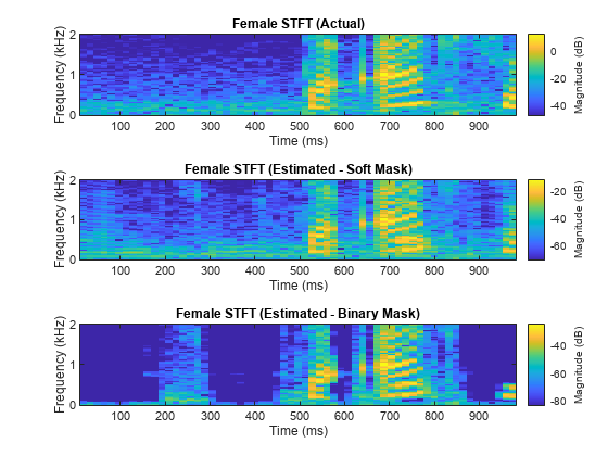
Compare STFTs of a one-second segment for mix, original female and male, and estimated female and male, respectively.

range = 7e4:7.4e4;

figure
stft(mixValidate(range),Fs,Window=win,OverlapLength=64,FFTLength=fftLength,FrequencyRange="onesided");
title("Mix STFT")

Figure contains an axes object. The axes object with title Mix STFT, xlabel Time (ms), ylabel Frequency (kHz) contains an object of type image.

figure
tiledlayout(3,1)

nexttile
stft(mSpeechValidate(range),Fs,Window=win,OverlapLength=64,FFTLength=fftLength,FrequencyRange="onesided");
title("Male STFT (Actual)")

nexttile
stft(maleSpeech_est_soft(range),Fs,Window=win,OverlapLength=64,FFTLength=fftLength,FrequencyRange="onesided");
title("Male STFT (Estimated - Soft Mask)")

nexttile
stft(maleSpeech_est_hard(range),Fs,Window=win,OverlapLength=64,FFTLength=fftLength,FrequencyRange="onesided");
title("Male STFT (Estimated - Binary Mask)");

figure
tiledlayout(3,1)

nexttile
stft(fSpeechValidate(range),Fs,Window=win,OverlapLength=64,FFTLength=fftLength,FrequencyRange="onesided");
title("Female STFT (Actual)")

nexttile
stft(femaleSpeech_est_soft(range),Fs,Window=win,OverlapLength=64,FFTLength=fftLength,FrequencyRange="onesided");
title("Female STFT (Estimated - Soft Mask)")

nexttile
stft(femaleSpeech_est_hard(range),Fs,Window=win,OverlapLength=64,FFTLength=fftLength,FrequencyRange="onesided");
title("Female STFT (Estimated - Binary Mask)")

References

[1] "Probabilistic Binary-Mask Cocktail-Party Source Separation in a Convolutional Deep Neural Network", Andrew J.R. Simpson, 2015.