Spectral Descriptors

Open Live Script

Signal Toolbox™ and Audio Toolbox™ provide a suite of functions that describe the shape, sometimes referred to as timbre, of audio. This example defines the equations used to determine the spectral features, cites common uses of each feature, and provides examples so that you can gain intuition about what the spectral descriptors are describing.

Spectral descriptors are widely used in machine and deep learning applications, and perceptual analysis. Spectral descriptors have been applied to a range of applications, including:

Speaker identification and recognition [21]
Acoustic scene recognition [11] [17]
Instrument recognition [22]
Music genre classification [16] [18]
Mood recognition [19] [20]
Voice activity detection [5] [7] [8] [10] [12] [13]

`Spectral Centroid`

The spectral centroid (spectralCentroid) is the frequency-weighted sum normalized by the unweighted sum [1]:

$μ_{1} = \frac{\sum_{k = b_{1}}^{b_{2}} f_{k} s_{k}}{\sum_{k = b_{1}}^{b_{2}} s_{k}}$

where

$f_{k}$ is the frequency in Hz corresponding to bin $k$ .
$s_{k}$ is the spectral value at bin $k$ . The magnitude spectrum and power spectrum are both commonly used.
$b_{1}$ and $b_{2}$ are the band edges, in bins, over which to calculate the spectral centroid.

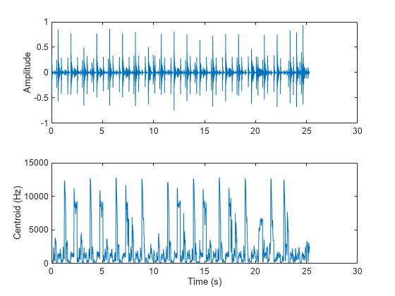
The spectral centroid represents the "center of gravity" of the spectrum. It is used as an indication of brightness [2] and is commonly used in music analysis and genre classification. For example, observe the jumps in the centroid corresponding to high hat hits in the audio file.

[audio,fs] = audioread('FunkyDrums-44p1-stereo-25secs.mp3');
audio = sum(audio,2)/2;

centroid = spectralCentroid(audio,fs);

subplot(2,1,1)
t = linspace(0,size(audio,1)/fs,size(audio,1));
plot(t,audio)
ylabel('Amplitude')

subplot(2,1,2)
t = linspace(0,size(audio,1)/fs,size(centroid,1));
plot(t,centroid)
xlabel('Time (s)')
ylabel('Centroid (Hz)')

Figure contains 2 axes objects. Axes object 1 with ylabel Amplitude contains an object of type line. Axes object 2 with xlabel Time (s), ylabel Centroid (Hz) contains an object of type line.

The spectral centroid is also commonly used to classify speech as voiced or unvoiced [3]. For example, the centroid jumps in regions of unvoiced speech.

[audio,fs] = audioread('Counting-16-44p1-mono-15secs.wav');

centroid = spectralCentroid(audio,fs);

subplot(2,1,1)
t = linspace(0,size(audio,1)/fs,size(audio,1));
plot(t,audio)
ylabel('Amplitude')

subplot(2,1,2)
t = linspace(0,size(audio,1)/fs,size(centroid,1));
plot(t,centroid)
xlabel('Time (s)')
ylabel('Centroid (Hz)')

Figure contains 2 axes objects. Axes object 1 with ylabel Amplitude contains an object of type line. Axes object 2 with xlabel Time (s), ylabel Centroid (Hz) contains an object of type line.

`Spectral Spread`

Spectral spread (spectralSpread) is the standard deviation around the spectral centroid [1]:

$μ_{2} = \sqrt{\frac{\sum_{k = b_{1}}^{b_{2}} {(f_{k} - μ_{1})}^{2} s_{k}}{\sum_{k = b_{1}}^{b_{2}} s_{k}}}$

where

$f_{k}$ is the frequency in Hz corresponding to bin $k$ .
$s_{k}$ is the spectral value at bin $k$ . The magnitude spectrum and power spectrum are both commonly used.
$b_{1}$ and $b_{2}$ are the band edges, in bins, over which to calculate the spectral spread.
$μ_{1}$ is the spectral centroid.

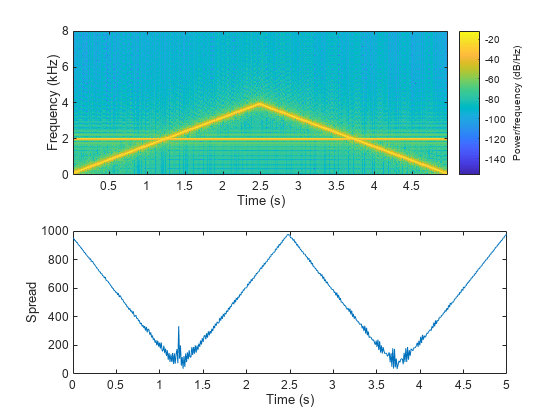
The spectral spread represents the "instantaneous bandwidth" of the spectrum. It is used as an indication of the dominance of a tone. For example, the spread increases as the tones diverge and decreases as the tones converge.

fs = 16e3;
tone = audioOscillator('SampleRate',fs,'NumTones',2,'SamplesPerFrame',512,'Frequency',[2000,100]);
duration = 5;
numLoops = floor(duration*fs/tone.SamplesPerFrame);
signal = [];
for i = 1:numLoops
    signal = [signal;tone()];
    if i<numLoops/2
        tone.Frequency = tone.Frequency + [0,50];
    else
        tone.Frequency = tone.Frequency - [0,50];
    end
end

spread = spectralSpread(signal,fs);

subplot(2,1,1)
spectrogram(signal,round(fs*0.05),round(fs*0.04),2048,fs,'yaxis')

subplot(2,1,2)
t = linspace(0,size(signal,1)/fs,size(spread,1));
plot(t,spread)
xlabel('Time (s)')
ylabel('Spread')

Figure contains 2 axes objects. Axes object 1 with xlabel Time (s), ylabel Frequency (kHz) contains an object of type image. Axes object 2 with xlabel Time (s), ylabel Spread contains an object of type line.

`Spectral Skewness`

Spectral skewness (spectralSkewness) is computed from the third order moment [1]:

$μ_{3} = \frac{\sum_{k = b_{1}}^{b_{2}} {(f_{k} - μ_{1})}^{3} s_{k}}{{(μ_{2})}^{3} \sum_{k = b_{1}}^{b_{2}} s_{k}}$

where

$f_{k}$ is the frequency in Hz corresponding to bin $k$ .
$s_{k}$ is the spectral value at bin $k$ . The magnitude spectrum and power spectrum are both commonly used.
$b_{1}$ and $b_{2}$ are the band edges, in bins, over which to calculate the spectral skewness.
$μ_{1}$ is the spectral centroid.
$μ_{2}$ is the spectral spread.

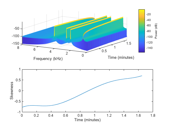
The spectral skewness measures symmetry around the centroid. In phonetics, spectral skewness is often referred to as spectral tilt and is used with other spectral moments to distinguish the place of articulation [4]. For harmonic signals, it indicates the relative strength of higher and lower harmonics. For example, in the four-tone signal, there is a positive skew when the lower tone is dominant and a negative skew when the upper tone is dominant.

fs = 16e3;
duration = 99;
tone = audioOscillator('SampleRate',fs,'NumTones',4,'SamplesPerFrame',fs,'Frequency',[500,2000,2500,4000],'Amplitude',[0,0.4,0.6,1]);

signal = [];
for i = 1:duration
    signal = [signal;tone()];
    tone.Amplitude = tone.Amplitude + [0.01,0,0,-0.01];
end

skewness = spectralSkewness(signal,fs);
t = linspace(0,size(signal,1)/fs,size(skewness,1))/60;

subplot(2,1,1)
spectrogram(signal,round(fs*0.05),round(fs*0.04),round(fs*0.05),fs,'yaxis','power')
view([-58 33])

subplot(2,1,2)
plot(t,skewness)
xlabel('Time (minutes)')
ylabel('Skewness')

Figure contains 2 axes objects. Axes object 1 with xlabel Time (minutes), ylabel Frequency (kHz) contains an object of type surface. Axes object 2 with xlabel Time (minutes), ylabel Skewness contains an object of type line.

`Spectral Kurtosis`

Spectral kurtosis (spectralKurtosis) is computed from the fourth order moment [1]:

$μ_{4} = \frac{\sum_{k = b_{1}}^{b_{2}} {(f_{k} - μ_{1})}^{4} s_{k}}{{(μ_{2})}^{4} \sum_{k = b_{1}}^{b_{2}} s_{k}}$

where

$f_{k}$ is the frequency in Hz corresponding to bin $k$ .
$s_{k}$ is the spectral value at bin $k$ . The magnitude spectrum and power spectrum are both commonly used.
$b_{1}$ and $b_{2}$ are the band edges, in bins, over which to calculate the spectral kurtosis.
$μ_{1}$ is the spectral centroid.
$μ_{2}$ is the spectral spread.

The spectral kurtosis measures the flatness, or non-Gaussianity, of the spectrum around its centroid. Conversely, it is used to indicate the peakiness of a spectrum. For example, as the white noise is increased on the speech signal, the kurtosis decreases, indicating a less peaky spectrum.

[audioIn,fs] = audioread('Counting-16-44p1-mono-15secs.wav');

noiseGenerator = dsp.ColoredNoise('Color','white','SamplesPerFrame',size(audioIn,1));

noise = noiseGenerator();
noise = noise/max(abs(noise));
ramp = linspace(0,.25,numel(noise))';
noise = noise.*ramp;

audioIn = audioIn + noise;

kurtosis = spectralKurtosis(audioIn,fs);

t = linspace(0,size(audioIn,1)/fs,size(audioIn,1));
subplot(2,1,1)
plot(t,audioIn)
ylabel('Amplitude')

t = linspace(0,size(audioIn,1)/fs,size(kurtosis,1));
subplot(2,1,2)
plot(t,kurtosis)
xlabel('Time (s)')
ylabel('Kurtosis')

Figure contains 2 axes objects. Axes object 1 with ylabel Amplitude contains an object of type line. Axes object 2 with xlabel Time (s), ylabel Kurtosis contains an object of type line.

`Spectral Entropy`

Spectral entropy (spectralEntropy) measures the peakiness of the spectrum [6]:

$entropy = \frac{- \sum_{k = b_{1}}^{b_{2}} s_{k} \log (s_{k})}{\log (b_{2} - b_{1})}$

where

$f_{k}$ is the frequency in Hz corresponding to bin $k$ .
$s_{k}$ is the spectral value at bin $k$ . The magnitude spectrum and power spectrum are both commonly used.
$b_{1}$ and $b_{2}$ are the band edges, in bins, over which to calculate the spectral entropy.

Spectral entropy has been used successfully in voiced/unvoiced decisions for automatic speech recognition [6]. Because entropy is a measure of disorder, regions of voiced speech have lower entropy compared to regions of unvoiced speech.

[audioIn,fs] = audioread('Counting-16-44p1-mono-15secs.wav');

entropy = spectralEntropy(audioIn,fs);

t = linspace(0,size(audioIn,1)/fs,size(audioIn,1));
subplot(2,1,1)
plot(t,audioIn)
ylabel('Amplitude')

t = linspace(0,size(audioIn,1)/fs,size(entropy,1));
subplot(2,1,2)
plot(t,entropy)
xlabel('Time (s)')
ylabel('Entropy')

Figure contains 2 axes objects. Axes object 1 with ylabel Amplitude contains an object of type line. Axes object 2 with xlabel Time (s), ylabel Entropy contains an object of type line.

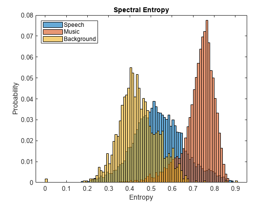
Spectral entropy has also been used to discriminate between speech and music [7] [8]. For example, compare histograms of entropy for speech, music, and background audio files.

fs = 8000;
[speech,speechFs] = audioread('Rainbow-16-8-mono-114secs.wav');
speech = resample(speech,fs,speechFs);
speech = speech./max(speech);

[music,musicFs] = audioread('RockGuitar-16-96-stereo-72secs.flac');
music = sum(music,2)/2;
music = resample(music,fs,musicFs);
music = music./max(music);

[background,backgroundFs] = audioread('Ambiance-16-44p1-mono-12secs.wav');
background = resample(background,fs,backgroundFs);
background = background./max(background);

speechEntropy     = spectralEntropy(speech,fs);
musicEntropy      = spectralEntropy(music,fs);
backgroundEntropy = spectralEntropy(background,fs);

figure
h1 = histogram(speechEntropy);
hold on
h2 = histogram(musicEntropy);
h3 = histogram(backgroundEntropy);

h1.Normalization = 'probability';
h2.Normalization = 'probability';
h3.Normalization = 'probability';
h1.BinWidth = 0.01;
h2.BinWidth = 0.01;
h3.BinWidth = 0.01;
title('Spectral Entropy')
legend('Speech','Music','Background','Location',"northwest")
xlabel('Entropy')
ylabel('Probability')
hold off

Figure contains an axes object. The axes object with title Spectral Entropy, xlabel Entropy, ylabel Probability contains 3 objects of type histogram. These objects represent Speech, Music, Background.

`Spectral Flatness`

Spectral flatness (spectralFlatness) measures the ratio of the geometric mean of the spectrum to the arithmetic mean of the spectrum [9]:

$flatness = \frac{{(\prod_{k = b_{1}}^{b_{2}} s_{k})}^{\frac{1}{b_{2} - b_{1}}}}{\frac{1}{b_{2} - b_{1}} \sum_{k = b_{1}}^{b_{2}} s_{k}}$

where

$s_{k}$ is the spectral value at bin $k$ . The magnitude spectrum and power spectrum are both commonly used.
$b_{1}$ and $b_{2}$ are the band edges, in bins, over which to calculate the spectral flatness.

Spectral flatness is an indication of the peakiness of the spectrum. A higher spectral flatness indicates noise, while a lower spectral flatness indicates tonality.

[audio,fs] = audioread('WaveGuideLoopOne-24-96-stereo-10secs.aif');
audio = sum(audio,2)/2;

noise = (2*rand(numel(audio),1)-1).*linspace(0,0.05,numel(audio))';

audio = audio + noise;

flatness = spectralFlatness(audio,fs);

subplot(2,1,1)
t = linspace(0,size(audio,1)/fs,size(audio,1));
plot(t,audio)
ylabel('Amplitude')

subplot(2,1,2)
t = linspace(0,size(audio,1)/fs,size(flatness,1));
plot(t,flatness)
ylabel('Flatness')
xlabel('Time (s)')

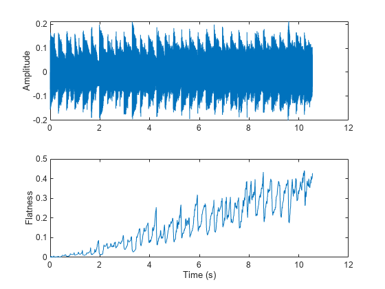
Figure contains 2 axes objects. Axes object 1 with ylabel Amplitude contains an object of type line. Axes object 2 with xlabel Time (s), ylabel Flatness contains an object of type line.

Spectral flatness has also been applied successfully to singing voice detection [10] and to audio scene recognition [11].

`Spectral Crest`

Spectral crest (spectralCrest) measures the ratio of the maximum of the spectrum to the arithmetic mean of the spectrum [1]:

$crest = \frac{\max (s_{k ϵ [b_{1}, b_{2}]})}{\frac{1}{b_{2} - b_{1}} \sum_{k = b_{1}}^{b_{2}} s_{k}}$

where

$s_{k}$ is the spectral value at bin $k$ . The magnitude spectrum and power spectrum are both commonly used.
$b_{1}$ and $b_{2}$ are the band edges, in bins, over which to calculate the spectral crest.

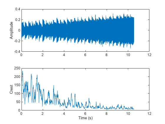
Spectral crest is an indication of the peakiness of the spectrum. A higher spectral crest indicates more tonality, while a lower spectral crest indicates more noise.

[audio,fs] = audioread('WaveGuideLoopOne-24-96-stereo-10secs.aif');
audio = sum(audio,2)/2;

noise = (2*rand(numel(audio),1)-1).*linspace(0,0.2,numel(audio))';

audio = audio + noise;

crest = spectralCrest(audio,fs);

subplot(2,1,1)
t = linspace(0,size(audio,1)/fs,size(audio,1));
plot(t,audio)
ylabel('Amplitude')

subplot(2,1,2)
t = linspace(0,size(audio,1)/fs,size(crest,1));
plot(t,crest)
ylabel('Crest')
xlabel('Time (s)')

Figure contains 2 axes objects. Axes object 1 with ylabel Amplitude contains an object of type line. Axes object 2 with xlabel Time (s), ylabel Crest contains an object of type line.

`Spectral Flux`

Spectral flux (spectralFlux) is a measure of the variability of the spectrum over time [12]:

$flux (t) = {(\sum_{k = b_{1}}^{b_{2}} {| s}_{k} (t) - s_{k} (t - 1) |^{p})}^{\frac{1}{p}}$

where

$s_{k}$ is the spectral value at bin $k$ . The magnitude spectrum and power spectrum are both commonly used.
$b_{1}$ and $b_{2}$ are the band edges, in bins, over which to calculate the spectral flux.
$p$ is the norm type.

Spectral flux is popularly used in onset detection [13] and audio segmentation [14]. For example, the beats in the drum track correspond to high spectral flux.

[audio,fs] = audioread('FunkyDrums-48-stereo-25secs.mp3');
audio = sum(audio,2)/2;

flux = spectralFlux(audio,fs);

subplot(2,1,1)
t = linspace(0,size(audio,1)/fs,size(audio,1));
plot(t,audio)
ylabel('Amplitude')

subplot(2,1,2)
t = linspace(0,size(audio,1)/fs,size(flux,1));
plot(t,flux)
ylabel('Flux')
xlabel('Time (s)')

Figure contains 2 axes objects. Axes object 1 with ylabel Amplitude contains an object of type line. Axes object 2 with xlabel Time (s), ylabel Flux contains an object of type line.

`Spectral Slope`

Spectral slope (spectralSlope) measures the amount of decrease of the spectrum [15]:

$slope = \frac{\sum_{k = b_{1}}^{b_{2}} (f_{k} - μ_{f}) (s_{k} - μ_{s})}{\sum_{k = b_{1}}^{b_{2}} {(f_{k} - μ_{f})}^{2}}$

where

$f_{k}$ is the frequency in Hz corresponding to bin $k$ .
$μ_{f}$ is the mean frequency.
$s_{k}$ is the spectral value at bin $k$ . The magnitude spectrum is commonly used.
$μ_{s}$ is the mean spectral value.
$b_{1}$ and $b_{2}$ are the band edges, in bins, over which to calculate the spectral slope.

Spectral slope has been used extensively in speech analysis, particularly in modeling speaker stress [19]. The slope is directly related to the resonant characteristics of the vocal folds and has also been applied to speaker identification [21]. Spectral slope is a socially important aspect of timbre. Spectral slope discrimination has been shown to occur in early childhood development [20]. Spectral slope is most pronounced when the energy in the lower formants is much greater than the energy in the higher formants.

[female,femaleFs] = audioread('FemaleSpeech-16-8-mono-3secs.wav');
female = female./max(female);


femaleSlope = spectralSlope(female,femaleFs);
t = linspace(0,size(female,1)/femaleFs,size(femaleSlope,1));
subplot(2,1,1)
spectrogram(female,round(femaleFs*0.05),round(femaleFs*0.04),round(femaleFs*0.05),femaleFs,'yaxis','power')

subplot(2,1,2)
plot(t,femaleSlope)
title('Female Speaker')
ylabel('Slope')
xlabel('Time (s)')

Figure contains 2 axes objects. Axes object 1 with xlabel Time (s), ylabel Frequency (kHz) contains an object of type image. Axes object 2 with title Female Speaker, xlabel Time (s), ylabel Slope contains an object of type line.

`Spectral Decrease`

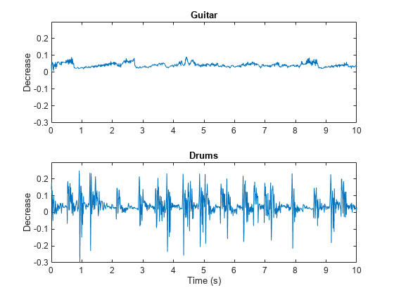
Spectral decrease (spectralDecrease) represents the amount of decrease of the spectrum, while emphasizing the slopes of the lower frequencies [1]:

$decrease = \frac{\sum_{k = b_{1} + 1}^{b_{2}} \frac{s_{k} - s_{b_{1}}}{k - 1}}{\sum_{k = b_{1} + 1}^{b_{2}} s_{k}}$

where

$s_{k}$ is the spectral value at bin $k$ . The magnitude spectrum is commonly used.
$b_{1}$ and $b_{2}$ are the band edges, in bins, over which to calculate the spectral decrease.

Spectral decrease is used less frequently than spectral slope in the speech literature, but it is commonly used, along with slope, in the analysis of music. In particular, spectral decrease has been shown to perform well as a feature in instrument recognition [22].

[guitar,guitarFs] = audioread('RockGuitar-16-44p1-stereo-72secs.wav');
guitar = mean(guitar,2);
[drums,drumsFs] = audioread('RockDrums-44p1-stereo-11secs.mp3');
drums = mean(drums,2);

guitarDecrease = spectralDecrease(guitar,guitarFs);
drumsDecrease = spectralDecrease(drums,drumsFs);

t1 = linspace(0,size(guitar,1)/guitarFs,size(guitarDecrease,1));
t2 = linspace(0,size(drums,1)/drumsFs,size(drumsDecrease,1));

subplot(2,1,1)
plot(t1,guitarDecrease)
title('Guitar')
ylabel('Decrease')
axis([0 10 -0.3 0.3])

subplot(2,1,2)
plot(t2,drumsDecrease)
title('Drums')
ylabel('Decrease')
xlabel('Time (s)')
axis([0 10 -0.3 0.3])

Figure contains 2 axes objects. Axes object 1 with title Guitar, ylabel Decrease contains an object of type line. Axes object 2 with title Drums, xlabel Time (s), ylabel Decrease contains an object of type line.

`Spectral Rolloff Point`

The spectral rolloff point (spectralRolloffPoint) measures the bandwidth of the audio signal by determining the frequency bin under which a given percentage of the total energy exists [12]:

$Rolloff Point = i such that \sum_{k = b_{1}}^{i} | s_{k} | = κ \sum_{k = b_{1}}^{b_{2}} s_{k}$

where

$s_{k}$ is the spectral value at bin $k$ . The magnitude spectrum and power spectrum are both commonly used.
$b_{1}$ and $b_{2}$ are the band edges, in bins, over which to calculate the spectral rolloff point.
$κ$ is the specified energy threshold, usually 95% or 85%.

$i$ is converted to Hz before it is returned by spectralRolloffPoint.

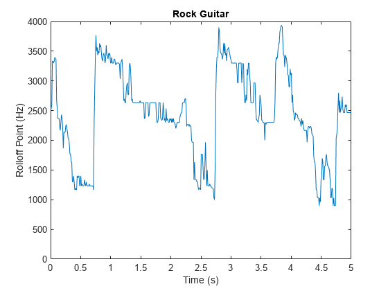
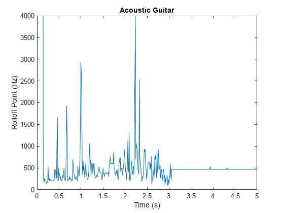
The spectral rolloff point has been used to distinguish between voiced and unvoiced speech, speech/music discrimination [12], music genre classification [16], acoustic scene recognition [17], and music mood classification [18]. For example, observe the different mean and variance of the rolloff point for speech, rock guitar, acoustic guitar, and an acoustic scene.

dur = 5; % Clip out 5 seconds from each file.

[speech,fs1] = audioread('SpeechDFT-16-8-mono-5secs.wav');
speech = speech(1:min(end,fs1*dur));

[electricGuitar,fs2] = audioread('RockGuitar-16-44p1-stereo-72secs.wav');
electricGuitar = mean(electricGuitar,2); % Convert to mono for comparison.
electricGuitar = electricGuitar(1:fs2*dur);

[acousticGuitar,fs3] = audioread('SoftGuitar-44p1_mono-10mins.ogg');
acousticGuitar = acousticGuitar(1:fs3*dur);

[acousticScene,fs4] = audioread('MainStreetOne-16-16-mono-12secs.wav');
acousticScene = acousticScene(1:fs4*dur);

r1 = spectralRolloffPoint(speech,fs1);
r2 = spectralRolloffPoint(electricGuitar,fs2);
r3 = spectralRolloffPoint(acousticGuitar,fs3);
r4 = spectralRolloffPoint(acousticScene,fs4);

t1 = linspace(0,size(speech,1)/fs1,size(r1,1));
t2 = linspace(0,size(electricGuitar,1)/fs2,size(r2,1));
t3 = linspace(0,size(acousticGuitar,1)/fs3,size(r3,1));
t4 = linspace(0,size(acousticScene,1)/fs4,size(r4,1));

figure
plot(t1,r1)
title('Speech')
ylabel('Rolloff Point (Hz)')
xlabel('Time (s)')
axis([0 5 0 4000])

Figure contains an axes object. The axes object with title Speech, xlabel Time (s), ylabel Rolloff Point (Hz) contains an object of type line.

figure
plot(t2,r2)
title('Rock Guitar')
ylabel('Rolloff Point (Hz)')
xlabel('Time (s)')
axis([0 5 0 4000])

Figure contains an axes object. The axes object with title Rock Guitar, xlabel Time (s), ylabel Rolloff Point (Hz) contains an object of type line.

figure
plot(t3,r3)
title('Acoustic Guitar')
ylabel('Rolloff Point (Hz)')
xlabel('Time (s)')
axis([0 5 0 4000])

Figure contains an axes object. The axes object with title Acoustic Guitar, xlabel Time (s), ylabel Rolloff Point (Hz) contains an object of type line.

figure
plot(t4,r4)
title('Acoustic Scene')
ylabel('Rolloff Point (Hz)')
xlabel('Time (s)')
axis([0 5 0 4000])

Figure contains an axes object. The axes object with title Acoustic Scene, xlabel Time (s), ylabel Rolloff Point (Hz) contains an object of type line.

References

[1] Peeters, G. "A Large Set of Audio Features for Sound Description (Similarity and Classification) in the CUIDADO Project." Technical Report; IRCAM: Paris, France, 2004.

[2] Grey, John M., and John W. Gordon. “Perceptual Effects of Spectral Modifications on Musical Timbres.” The Journal of the Acoustical Society of America. Vol. 63, Issue 5, 1978, pp. 1493–1500.

[3] Raimy, Eric, and Charles E. Cairns. The Segment in Phonetics and Phonology. Hoboken, NJ: John Wiley & Sons Inc., 2015.

[4] Jongman, Allard, et al. “Acoustic Characteristics of English Fricatives.” The Journal of the Acoustical Society of America. Vol. 108, Issue 3, 2000, pp. 1252–1263.

[5] S. Zhang, Y. Guo, and Q. Zhang, "Robust Voice Activity Detection Feature Design Based on Spectral Kurtosis." First International Workshop on Education Technology and Computer Science, 2009, pp. 269–272.

[6] Misra, H., S. Ikbal, H. Bourlard, and H. Hermansky. "Spectral Entropy Based Feature for Robust ASR." 2004 IEEE International Conference on Acoustics, Speech, and Signal Processing.

[7] A. Pikrakis, T. Giannakopoulos, and S. Theodoridis. "A Computationally Efficient Speech/Music Discriminator for Radio Recordings." International Conference on Music Information Retrieval and Related Activities, 2006.

[8] Pikrakis, A., et al. “A Speech/Music Discriminator of Radio Recordings Based on Dynamic Programming and Bayesian Networks.” IEEE Transactions on Multimedia. Vol. 10, Issue 5, 2008, pp. 846–857.

[9] Johnston, J.d. “Transform Coding of Audio Signals Using Perceptual Noise Criteria.” IEEE Journal on Selected Areas in Communications. Vol. 6, Issue 2, 1988, pp. 314–323.

[10] Lehner, Bernhard, et al. “On the Reduction of False Positives in Singing Voice Detection.” 2014 IEEE International Conference on Acoustics, Speech and Signal Processing (ICASSP), 2014.

[11] Y. Petetin, C. Laroche and A. Mayoue, "Deep Neural Networks for Audio Scene Recognition," 2015 23rd European Signal Processing Conference (EUSIPCO), 2015.

[12] Scheirer, E., and M. Slaney. “Construction and Evaluation of a Robust Multifeature Speech/Music Discriminator.” 1997 IEEE International Conference on Acoustics, Speech, and Signal Processing, 1997.

[13] S. Dixon, "Onset Detection Revisited." International Conference on Digital Audio Effects. Vol. 120, 2006, pp. 133–137.

[14] Tzanetakis, G., and P. Cook. “Multifeature Audio Segmentation for Browsing and Annotation.” Proceedings of the 1999 IEEE Workshop on Applications of Signal Processing to Audio and Acoustics, 1999.

[15] Lerch, Alexander. An Introduction to Audio Content Analysis Applications in Signal Processing and Music Informatics. Piscataway, NJ: IEEE Press, 2012.

[16] Li, Tao, and M. Ogihara. "Music Genre Classification with Taxonomy." IEEE International Conference on Acoustics, Speech, and Signal Processing, 2005.

[17] Eronen, A.j., V.t. Peltonen, J.t. Tuomi, A.p. Klapuri, S. Fagerlund, T. Sorsa, G. Lorho, and J. Huopaniemi. "Audio-Based Context Recognition." IEEE Transactions on Audio, Speech and Language Processing. Vol. 14, Issue 1, 2006, pp. 321–329.

[18] Ren, Jia-Min, Ming-Ju Wu, and Jyh-Shing Roger Jang. "Automatic Music Mood Classification Based on Timbre and Modulation Features." IEEE Transactions on Affective Computing. Vol. 6, Issue 3, 2015, pp. 236–246.

[19] Hansen, John H. L., and Sanjay Patil. "Speech Under Stress: Analysis, Modeling and Recognition." Lecture Notes in Computer Science. Vol. 4343, 2007, pp. 108–137.

[20] Tsang, Christine D., and Laurel J. Trainor. "Spectral Slope Discrimination in Infancy: Sensitivity to Socially Important Timbres." Infant Behavior and Development. Vol. 25, Issue 2, 2002, pp. 183–194.

[21] Murthy, H.a., F. Beaufays, L.p. Heck, and M. Weintraub. "Robust Text-Independent Speaker Identification over Telephone Channels." IEEE Transactions on Speech and Audio Processing. Vol. 7, Issue 5, 1999, pp. 554–568.

[22] Essid, S., G. Richard, and B. David. "Instrument Recognition in Polyphonic Music Based on Automatic Taxonomies." IEEE Transactions on Audio, Speech and Language Processing. Vol 14, Issue 1, 2006, pp. 68–80.