Differential Analysis of Complex Protein and Metabolite Mixtures Using Liquid Chromatography/Mass Spectrometry (LC/MS)

Introduction

The use of complex peptide and metabolite mixtures in LC/MS requires label-free alignment procedures. The analysis of this type of data requires searching for statistically significant differences between biologically related data sets, without the need for a full identification of all the compounds in the sample (either peptides/proteins or metabolites). Comparing compounds requires alignment in two dimensions, the mass-charge dimension and the retention time dimension [1]. In the examples Preprocessing Raw Mass Spectrometry Data and Visualizing and Preprocessing Hyphenated Mass Spectrometry Data Sets for Metabolite and Protein/Peptide Profiling, you can learn how to use the MSALIGN, MSPALIGN, and SAMPLEALIGN functions to warp or calibrate different type of anomalies in the mass/charge dimension. In this example, you will learn how to use the SAMPLEALIGN function to also correct the nonlinear and unpredicted variations in the retention time dimension.

While it is possible to implement alternative methods for aligning retention times, other approaches typically require identification of compounds, which is not always feasible, or manual manipulations that thwart attempts to automate for high throughput data analysis.

Data Set Description

This example uses two samples in PAe000153 and PAe000155 available from Peptide Atlas [2]. The samples are LC-ESI-MS scans of four salt protein fractions from the saccharomyces cerevisiae each containing more than 1000 peptides. Yeast samples were treated with different chemicals (glycine and serine) in order to get two biologically diverse samples. Time alignment of these two data sets is one of the most challenging cases reported in [3]. The data sets are not distributed with MATLAB®. You can try other data sets available in public databases for protein data, such as Peptide Atlas Repository. If you receive any errors related to memory or java heap space, try increasing your java heap space as described here. LC/MS data analysis requires extended amounts of memory from the operating system; if you receive "Out of memory" errors when running this example, try increasing the virtual memory (or swap space) of your operating system. For details, see Resolve “Out of Memory” Errors.

Read and extract the lists of peaks from the XML files containing the intensity data for the sample treated with Serine and the sample treated with Glycine.

ser = mzxmlread('005_1.mzXML')
[ps,ts] = mzxml2peaks(ser,'level',1);
gly = mzxmlread('005a.mzXML')
[pg,tg] = mzxml2peaks(gly,'level',1);

ser = 

  struct with fields:

     scan: [5610×1 struct]
    mzXML: [1×1 struct]
    index: [1×1 struct]


gly = 

  struct with fields:

     scan: [5518×1 struct]
    mzXML: [1×1 struct]
    index: [1×1 struct]

Use the MSPPRESAMPLE function to resample the data sets while preserving the peak heights and locations in the mass/charge dimension. Data sets are resampled to have both a common grid with 5,000 mass/charge values. A common grid is desirable for comparative visualization, and for differential analysis.

[MZs,Ys] = msppresample(ps,5000);
[MZg,Yg] = msppresample(pg,5000);

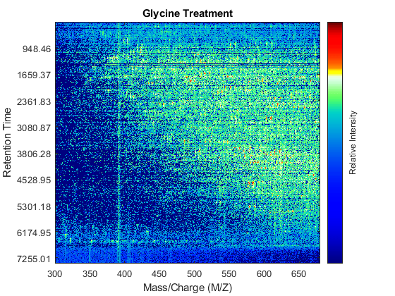
Use the MSHEATMAP function to visualize both samples. When working with heat maps it is a common technique to display the logarithm of the ion intensities, which enhances the dynamic range of the colormap.

fh1 = msheatmap(MZs,ts,log(Ys),'resolution',0.15);
title('Serine Treatment')
fh2 = msheatmap(MZg,tg,log(Yg),'resolution',0.15);
title('Glycine Treatment')

Detailed Inspection of the Misalignment Problems

Notice you can visualize the data sets separately; however, the time vectors have different size, and therefore the heat maps have different number of rows (or Ys and Yg have different number of columns). Moreover, the sampling rate is not constant and the shift between the time vectors is not linear.

whos('Ys','Yg','ts','tg')
figure
plot(1:numel(ts),ts,1:numel(tg),tg)
legend('Serine','Glycine','Location','NorthWest')
title('Time Vectors')
xlabel('Spectrum Index')
ylabel('Retention Time (seconds)')

  Name         Size                Bytes  Class     Attributes

  Yg        5000x921            18420000  single              
  Ys        5000x937            18740000  single              
  tg         921x1                  7368  double              
  ts         937x1                  7496  double              

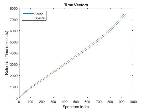
To observe the same region of interest in both data sets, you need to calculate the appropriate row indices in each matrix. For example, to inspect the peptide peaks in the 480-520 Da MZ range and 1550-1900 seconds retention time range, you need to find the closest matches for this range in the time vectors and then zoom in each figure:

ind_ser = samplealign(ts,[1550;1900]);
figure(fh1);
axis([480 520 ind_ser'])

ind_gly = samplealign(tg,[1550;1900]);
figure(fh2);
axis([480 520 ind_gly'])

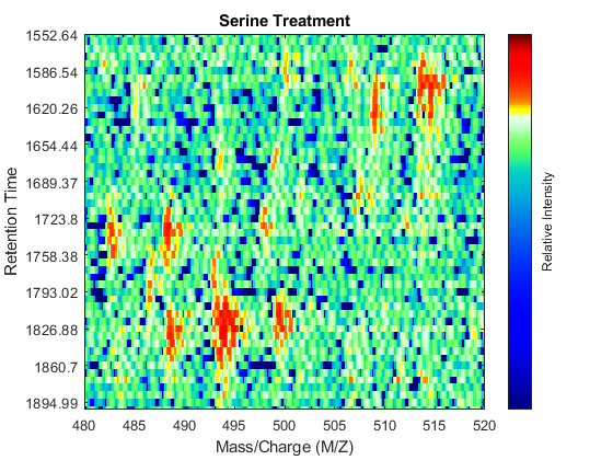
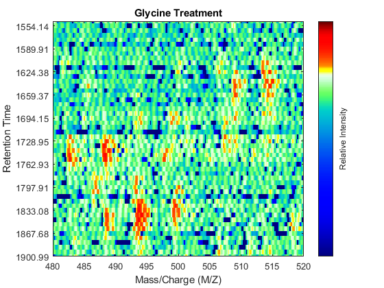
Even though you zoomed in the same range, you can still observe that the top-right peptide in the axes is shifted in the retention time dimension. In the sample treated with serine, the center of this peak appears to occur at approximately 1595 seconds, while in the sample treated with glycine the putative same peptide occurs at approximately 1630 seconds. This will prevent you from a accurate comparative analysis, even if you resample the data sets to the same time vector. In addition to the shift in the retention time, the data set seems to be improperly calibrated in the mass/charge dimension, because the peaks do not have a compact shape in contiguous spectra.

Mass/Charge Calibration and Enhancement of the Matrices

Before correcting the retention time, you can enhance the samples using an approach similar to the one described in the example Visualizing and Preprocessing Hyphenated Mass Spectrometry Data Sets for Metabolite and Protein/Peptide Profiling. For brevity, we only display the MATLAB code without any further explanation:

SF = @(x) 1-exp(-x./5e7); % scaling function
DF = @(R,S) sqrt((SF(R(:,2))-SF(S(:,2))).^2 + (R(:,1)-S(:,1)).^2);
CMZ = (315:.10:680)'; % Common Mass/Charge Vector with a finer grid

% Align peaks of the serine sample in the MZ direction
LAI = zeros(size(CMZ));
for i = 1:numel(ps)
    if ~rem(i,250), fprintf(' %d...',i); end
    [k,j] = samplealign([CMZ,LAI],double(ps{i}),'band',1.5,'gap',[0 2],'dist',DF);
    LAI = LAI*.25;
    LAI(k) = LAI(k) + ps{i}(j,2);
    psa{i,1} = [CMZ(k) ps{i}(j,2)];
end

% Align peaks of the glycine sample in the MZ direction
LAI = zeros(size(CMZ));
for i = 1:numel(pg)
    if ~rem(i,250), fprintf(' %d...',i); end
    [k,j] = samplealign([CMZ,LAI],double(pg{i}),'band',1.5,'gap',[0 2],'dist',DF);
    LAI = LAI*.25;
    LAI(k) = LAI(k) + pg{i}(j,2);
    pga{i,1} = [CMZ(k) pg{i}(j,2)];
end

% Peak-preserving resample
[MZs,Ys] = msppresample(psa,5000);
[MZg,Yg] = msppresample(pga,5000);

% Gaussian Filtering
Gpulse = exp(-.5*(-10:10).^2)./sum(exp(-.05*(-10:10).^2));
Ysf = convn(Ys,Gpulse,'same');
Ygf = convn(Yg,Gpulse,'same');

% Visualization
fh3 = msheatmap(MZs,ts,log(Ysf),'resolution',0.15);
title('Serine Treatment (Enhanced)')
axis([480 520 ind_ser'])
fh4 = msheatmap(MZg,tg,log(Ygf),'resolution',0.15);
title('Glycine Treatment (Enhanced)')
axis([480 520 ind_gly'])

 250... 500... 750... 250... 500... 750...

Chromatographic Alignment

At this point, you have mass/charge calibrated and smoothed the two LC/MS data sets, but you are still unable to perform a differential analysis because the data sets have a small misalignment along the retention time axis.

You can use SAMPLEALIGN to correct the drift in the chromatographic domain. First, you should inspect the data and look for the worst case shift, this helps you to estimate the BAND constraint. By panning over both heat maps you can observe that common peptide peaks are not shifted more than 50 seconds. Use the input argument SHOWCONSTRAINTS to display the constraint space for the time warping operation and assess if the Dynamic Programming (DP) algorithm can handle this problem size. In this case you have less than 12,000 nodes. By omitting the output arguments, SAMPLEALIGN displays only the constraints without running the DP algorithm. Also note that the input signals are the filtered and enhanced data sets, but these have been upsampled to 5,000 MZ values, which are very computationally demanding if you use all. Therefore, use the function MSPALIGN to obtain a reduced list of mass/charge values (RMZ) indicating where the most intense peaks are, then use the SAMPLEALIGN function also to find the indices of MZs (or MZg) that best match the reduced mass/charge vector:

RMZ = mspalign([ps;pg])';
idx = samplealign(MZs,RMZ,'width',1); % with these input parameters this
                                      % operation is equivalent to find the
                                      % nearest neighbor for each RMZ in
                                      % MZs.

samplealign([ts Ysf(idx,:)'],[tg Ygf(idx,:)'],'band',50,'showconstraints',true)

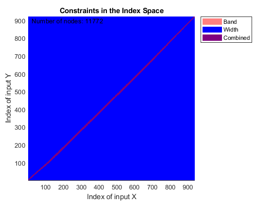
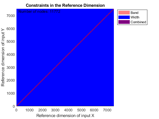
SAMPLEALIGN uses the Euclidean distance as default to score matched pairs of samples. In LC/MS data sets each sample corresponds to a spectrum at a given time, therefore, the cross-correlation between each pair of matched spectra provides a better distance metric. SAMPLEALIGN allows you to define your own metric to calculate the distance between spectra, it is also possible to envision a metric that rewards more spectra pairs that match high ion intensity peaks rather than low ion intensity noisy peaks. Use the input argument WEIGHT to remove the first column from the inputs, which represents the retention time, so the scoring metric between spectra is based only on the ion intensities.

cc = @(Xu,Yu) (mean(Xu.*Yu,2).^2)./mean(Xu.*Xu,2)./mean(Yu.*Yu,2);
ub = @(X) bsxfun(@minus,X,mean(X,2));
df = @(x,y) 1-cc(ub(x),ub(y));

[i,j] = samplealign([ts Ysf(idx,:)'],[tg Ygf(idx,:)'],'band',50,...
                    'distance',df ,'weight',[false true(1,numel(idx))]);

fh5 = figure;
plot(ts(i),tg(j)); grid
title('Warp Function')
xlabel('Retention Time in Data Set with Serine')
ylabel('Retention Time in Data Set with Glycine')

fh6 = figure; hold on
plot((ts(i)+tg(j))/2,ts(i)-tg(j))
title('Shift Function')
xlabel('Retention Time')
ylabel('Retention Time Shift between Data Sets')

Because it is expected that the real shift function between both data sets is continuous, you can smooth the observed shifts or regress a continuous model to create a warp model between the two time axes. In this example, we simply regress the drifting to a polynomial function:

[p,p_struct,mu] = polyfit((ts(i)+tg(j))/2,ts(i)-tg(j),20);
sf = @(z) polyval(p,(z-mu(1))./mu(2));
figure(fh6)
plot(tg,sf(tg),'r')
legend('Observed shifts','Estimated shift curve','Location','SouthEast')

Comparative Analysis

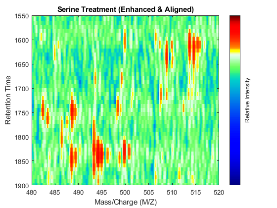
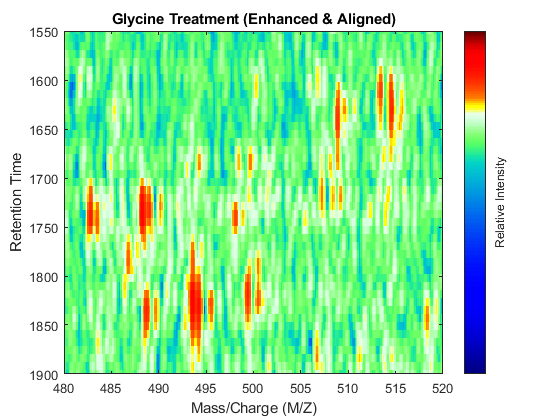
To carry out a comparative analysis, resample the LC/MS data sets to a common time vector. When resampling we use the estimated shift function to correct the retention time dimension. In this example, each spectrum in both data sets is shifted half the distance of the shift function. In the case of multiple alignment of data sets, it is possible to calculate the pairwise shift functions between all data sets, and then apply the corrections to a common reference in such a way that the overall shifts are minimized [4].

t = (max(min(tg),min(ts)):mean(diff(tg)):min(max(tg),max(ts)))';

% Visualization
fh7 = msheatmap(MZs,t,log(interp1q(ts,Ysf',t+sf(t)/2)'),'resolution',0.15);
title('Serine Treatment (Enhanced & Aligned)')
fh8 = msheatmap(MZg,t,log(interp1q(tg,Ygf',t-sf(t)/2)'),'resolution',0.15);
title('Glycine Treatment (Enhanced & Aligned)')

To interactively or programmatically compare regions between two enhanced and time aligned data sets, you can link the axes of two heat maps. Because the heat maps now use a regularly spaced time vector, you can zoom in by using the AXIS function without having to search the appropriate row indices of the matrices.

linkaxes(findobj([fh7 fh8],'Tag','MSHeatMap'))
axis([480 520 1550 1900])

References

[1] Listgarten, J. and Emili, A., "Statistical and computational methods for comparative proteomic profiling using liquid chromatography tandem mass spectrometry", Molecular and Cell Proteomics, 4(4):419-34, 2005.

[2] Desiere, F., et al., "The Peptide Atlas Project", Nucleic Acids Research, 34:D655-8, 2006.

[3] Prince, J.T. and Marcotte, E.M., "Chromatographic alignment of ESI-LC-MS proteomics data sets by ordered bijective interpolated warping", Analytical Chemistry, 78(17):6140-52, 2006.

[4] Andrade L. and Manolakos E.S., "Automatic Estimation of Mobility Shift Coefficients in DNA Chromatograms", Neural Networks for Signal Processing Proceedings, 91-100, 2003.