Exploring Protein-DNA Binding Sites from Paired-End ChIP-Seq Data

Open Script

This example shows how to perform a genome-wide analysis of a transcription factor in the Arabidopsis Thaliana (Thale Cress) model organism.

For enhanced performance, it is recommended that you run this example on a 64-bit platform, because the memory footprint is close to 2 Gb. On a 32-bit platform, if you receive "Out of memory" errors when running this example, try increasing the virtual memory (or swap space) of your operating system or try setting the 3GB switch (32-bit Windows® XP only). For details, see Resolve “Out of Memory” Errors.

Introduction

ChIP-Seq is a technology that is used to identify transcription factors that interact with specific DNA sites. First chromatin immunoprecipitation enriches DNA-protein complexes using an antibody that binds to a particular protein of interest. Then, all the resulting fragments are processed using high-throughput sequencing. Sequencing fragments are mapped back to the reference genome. By inspecting over-represented regions it is possible to mark the genomic location of DNA-protein interactions.

In this example, short reads are produced by the paired-end Illumina® platform. Each fragment is reconstructed from two short reads successfully mapped, with this the exact length of the fragment can be computed. Using paired-end information from sequence reads maximizes the accuracy of predicting DNA-protein binding sites.

Data Set

This example explores the paired-end ChIP-Seq data generated by Wang et.al. [1] using the Illumina® platform. The data set has been courteously submitted to the Gene Expression Omnibus repository with accession number GSM424618. The unmapped paired-end reads can be obtained from the NCBI FTP site.

This example assumes that you:

(1) downloaded the data containing the unmapped short read and converted it to FASTQ formatted files using the NCBI SRA Toolkit.

(2) produced a SAM formatted file by mapping the short reads to the Thale Cress reference genome, using a mapper such as BWA [2], Bowtie, or SSAHA2 (which is the mapper used by authors of [1]), and,

(3) ordered the SAM formatted file by reference name first, then by genomic position.

For the published version of this example, 8,655,859 paired-end short reads are mapped using the BWA mapper [2]. BWA produced a SAM formatted file (aratha.sam) with 17,311,718 records (8,655,859 x 2). Repetitive hits were randomly chosen, and only one hit is reported, but with lower mapping quality. The SAM file was ordered and converted to a BAM formatted file using SAMtools [3] before being loaded into MATLAB.

The last part of the example also assumes that you downloaded the reference genome for the Thale Cress model organism (which includes five chromosomes). Uncomment the following lines of code to download the reference from the NCBI repository:

% getgenbank('NC_003070','FileFormat','fasta','tofile','ach1.fasta');
% getgenbank('NC_003071','FileFormat','fasta','tofile','ach2.fasta');
% getgenbank('NC_003074','FileFormat','fasta','tofile','ach3.fasta');
% getgenbank('NC_003075','FileFormat','fasta','tofile','ach4.fasta');
% getgenbank('NC_003076','FileFormat','fasta','tofile','ach5.fasta');

Creating a MATLAB® Interface to a BAM Formatted File

To create local alignments and look at the coverage we need to construct a BioMap. BioMap has an interface that provides direct access to the mapped short reads stored in the BAM formatted file, thus minimizing the amount of data that is actually loaded to the workspace. Create a BioMap to access all the short reads mapped in the BAM formatted file.

bm = BioMap('aratha.bam')

bm = 

  BioMap with properties:

    SequenceDictionary: {5x1 cell}
             Reference: [14637324x1 File indexed property]
             Signature: [14637324x1 File indexed property]
                 Start: [14637324x1 File indexed property]
        MappingQuality: [14637324x1 File indexed property]
                  Flag: [14637324x1 File indexed property]
          MatePosition: [14637324x1 File indexed property]
               Quality: [14637324x1 File indexed property]
              Sequence: [14637324x1 File indexed property]
                Header: [14637324x1 File indexed property]
                 NSeqs: 14637324
                  Name: ''

Use the getSummary method to obtain a list of the existing references and the actual number of short read mapped to each one.

getSummary(bm)

BioMap summary:
                                  Name: ''
                        Container_Type: 'Data is file indexed.'
             Total_Number_of_Sequences: 14637324
    Number_of_References_in_Dictionary: 5

            Number_of_Sequences    Genomic_Range 
    Chr1    3151847                   1  30427671
    Chr2    3080417                1000  19698292
    Chr3    3062917                  94  23459782
    Chr4    2218868                1029  18585050
    Chr5    3123275                  11  26975502

The remainder of this example focuses on the analysis of one of the five chromosomes, Chr1. Create a new BioMap to access the short reads mapped to the first chromosome by subsetting the first one.

bm1 = getSubset(bm,'SelectReference','Chr1')

bm1 = 

  BioMap with properties:

    SequenceDictionary: 'Chr1'
             Reference: [3151847x1 File indexed property]
             Signature: [3151847x1 File indexed property]
                 Start: [3151847x1 File indexed property]
        MappingQuality: [3151847x1 File indexed property]
                  Flag: [3151847x1 File indexed property]
          MatePosition: [3151847x1 File indexed property]
               Quality: [3151847x1 File indexed property]
              Sequence: [3151847x1 File indexed property]
                Header: [3151847x1 File indexed property]
                 NSeqs: 3151847
                  Name: ''

By accessing the Start and Stop positions of the mapped short read you can obtain the genomic range.

x1 = min(getStart(bm1))
x2 = max(getStop(bm1))

x1 =

  uint32

   1


x2 =

  uint32

   30427671

Exploring the Coverage at Different Resolutions

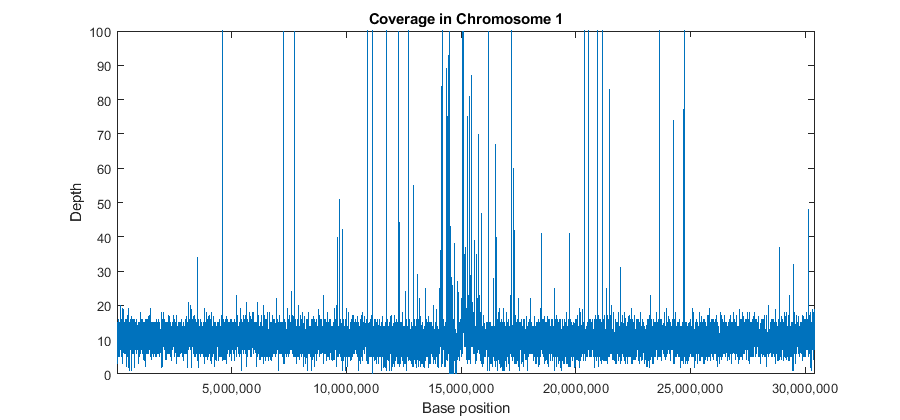
To explore the coverage for the whole range of the chromosome, a binning algorithm is required. The getBaseCoverage method produces a coverage signal based on effective alignments. It also allows you to specify a bin width to control the size (or resolution) of the output signal. However internal computations are still performed at the base pair (bp) resolution. This means that despite setting a large bin size, narrow peaks in the coverage signal can still be observed. Once the coverage signal is plotted you can program the figure's data cursor to display the genomic position when using the tooltip. You can zoom and pan the figure to determine the position and height of the ChIP-Seq peaks.

[cov,bin] = getBaseCoverage(bm1,x1,x2,'binWidth',1000,'binType','max');
figure
plot(bin,cov)
axis([x1,x2,0,100])        % sets the axis limits
fixGenomicPositionLabels   % formats tick labels and adds datacursors
xlabel('Base position')
ylabel('Depth')
title('Coverage in Chromosome 1')

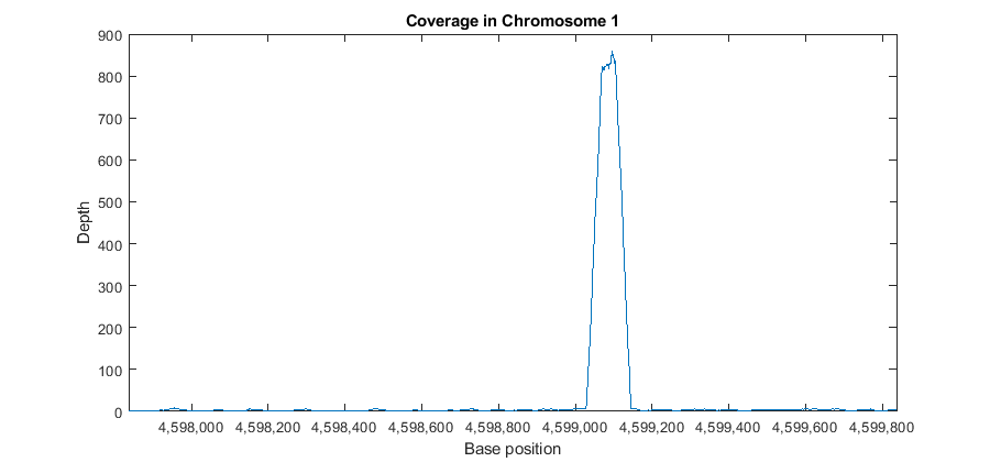
It is also possible to explore the coverage signal at the bp resolution (also referred to as the pile-up profile). Explore one of the large peaks observed in the data at position 4598837.

p1 = 4598837-1000;
p2 = 4598837+1000;

figure
plot(p1:p2,getBaseCoverage(bm1,p1,p2))
xlim([p1,p2])              % sets the x-axis limits
fixGenomicPositionLabels   % formats tick labels and adds datacursors
xlabel('Base position')
ylabel('Depth')
title('Coverage in Chromosome 1')

Identifying and Filtering Regions with Artifacts

Observe the large peak with coverage depth of 800+ between positions 4599029 and 4599145. Investigate how these reads are aligning to the reference chromosome. You can retrieve a subset of these reads enough to satisfy a coverage depth of 25, since this is sufficient to understand what is happening in this region. Use getIndex to obtain indices to this subset. Then use getCompactAlignment to display the corresponding multiple alignment of the short-reads.

i = getIndex(bm1,4599029,4599145,'depth',25);
bmx = getSubset(bm1,i,'inmemory',false)
getCompactAlignment(bmx,4599029,4599145)

bmx = 

  BioMap with properties:

    SequenceDictionary: 'Chr1'
             Reference: [62x1 File indexed property]
             Signature: [62x1 File indexed property]
                 Start: [62x1 File indexed property]
        MappingQuality: [62x1 File indexed property]
                  Flag: [62x1 File indexed property]
          MatePosition: [62x1 File indexed property]
               Quality: [62x1 File indexed property]
              Sequence: [62x1 File indexed property]
                Header: [62x1 File indexed property]
                 NSeqs: 62
                  Name: ''



ans =

  35×117 char array

    'AGTT AATCAAATAGAAAGCCCCGAGGGCGCCATATCCTAGGCGC  AAACTATGTGATTGAATAAATCCTCCTCTATCTGTTGCGG   GAGGACTCCTTCTCCTTCCCCTTTTGG'
    'AGTGC  TCAAATAGAAAGCCCCGAGGGCGCCATATTCTAGGAGCCC             GAATAAATCCTCCTCTATCTGTTGCGGGTCGAGGACTCCT CTCCTGCCCCTTTTGG'
    'AGTTCAA             CCCGAGGGCGCCATATTCTAGGAGCCCAAACTATGTGATT               TATCTGTTGCGGGTCGAGGACTCCTTCTCCTTCCCCTTCT  '
    'AGTTCAATCAAATAGAAAGC               TTCTAGGAGCCCAAACTATGTGATTGAATAAATCCTCCTC                AGGACTCCTTCTCCTTCCCCTTTTGG'
    'AGTT                                  AAGGAGCCCAAAATATGTGATTGAATAAATCCACCTCTAT              GGACTCCTTCTCCTTCCCCTTTTGG'
    'AGTACAATCAAATAGAAAGCCCCGAGGGCGCCATA   TAGGAGCCCAAACTATGTGATTGAATAAATCCTCCTCTAT                   CCTTCACCTTCCCCTTTTGG'
    'CGTACAATCAAATAGAAAGCCCCGAGGGCGCCATATTC  GGAGCCCAAACTATGTGATTGAATAAATCCTCCTCTATCT                         TTCCCCTTTTGG'
    'CGTACAATCAAATAGAAAGCCCCGAGGGCGCCATATTC  GGAGCCCAAACTATGTGATTGAATAAATCCTCCTCTATCT                                     '
    'CGTACAATCAAATAGAAAGCCCCGAGGGCGCCATATTC  GGAGCCCAAGCTATGTGATTGAATAAATCCTCCTCTATCT                                     '
    'CGTACAATCAAATAGAAAGCCCCGAGGGCGCCATATTC  GGAGCCCAAACTATGTGATTGAATAAATCCTCCTCTATCT                                     '
    'AGTTCAATCAAATAGAAAGCCCCGAGGGCGCCATATTCTA GAGCCCAAACTATGTGATTGAATAAATCCTCCTCTATCTG                                    '
    'GATACAATCAAATAGAAAGCCCCGAGGGCGCCATATTCTA GAGCCCAAACTATGTGATTGAATAAATCTTCCTCTATCTG                                    '
    'GATACAATCAAATAGAAAGCCCCGAGGGCGCCATATTCTA GAGCCCAAACTATGTGATTGAATAAATCCTCCTCTATCTG                                    '
    'GATACAATCAAATAGAAAGCCCCGAGGGCGCCATATTCTA GAGCCCAAACTATGTGATTGAATAAATCCTCCTCTATCTG                                    '
    'GATACAATCAAATAGAAAGCCCCGAGGGCGCCATATTCTA GAGCCCAAATTATGTGATTGAATAAATCCTCCTCTATCTG                                    '
    ' ATACAATCAAATAGAAAGCCCCGAGGGCGCCATATTCTAG   CCCAAACTATGTGATTGAATAAATCCTCCTCTATCTGTTG                                 '
    ' ATACAATCAAATAGAAAGCCCCGAGGGCGCCATATTCTAG   CACAAACTATGTGATTGAATAAATCCTCCTCTATCTGTTG                                 '
    ' ATACAATCAAATAGAAAGCCCCGAGGGCGCCATATTCTAG    CCAAACTATGTGATTGAATAAATCCTCCTCTATCTGTTGC                                '
    ' ATACAATCAAATAGAAAGCCCCGAGGGCGCCATATTCTAG                                                                            '
    ' ATACAATCAAATAGAAAGCCCCGAGGGCGCCATATTCTCG                                                                            '
    ' ATACAATCAAATAGAAAGCCCCGGGGGCGCCATATTCTAG                                                                            '
    ' ATTGAGTCAAATAGAAAGCCCCGAGGGCGCCATATTCTAG                                                                            '
    ' ATACAATCAAATAGAAAGCCCCGAGGGCGCCATATTCTAG                                                                            '
    ' ATACAATCAAATAGAAAGCCCCGAGGGCGCCATATTCTAG                                                                            '
    ' ATACAATCAAATAGAAAGCCCCGAGGGCGCCATATTCTAG                                                                            '
    '    CAATCAAATAGAAAGCCCCGAGGGCGCCATATTCTAGGAG                                                                         '
    '    CAATCAAATAGAAAGCCCCGAGGGCGCCATATTCTAGGAG                                                                         '
    '                                      TAGGAGCCCAAACTATGTGATTGAATAAATCCTCCTCTAT                                       '
    '                                      TAGGAGCCCAAACTATGCCATTGAATAAATCCTCCGCTAT                                       '
    '                                        GGAGCCCAAGCTATGTGATTGAATAAATCCTCCTCTATCT                                     '
    '                                         GAGCCCAAACTATGTGATTGAATAAATCCTCCTCTATCTG                                    '
    '                                         GAGCCCAAACTATGTGATTGAATAAATCCTCCTCTATCTG                                    '
    '                                         GAGCCCAAACTATGTGATTGAATAAATCCTCCTCTATCTG                                    '
    '                                         GAGCCCAAACTATGTGATTGAATAAATCCTCCTCTATCTG                                    '
    '                                         GAGCCCAAACTATGTGATTGAATAAATCCTCCTCTATCTG                                    '

In addition to visually confirming the alignment, you can also explore the mapping quality for all the short reads in this region, as this may hint to a potential problem. In this case, less than one percent of the short reads have a Phred quality of 60, indicating that the mapper most likely found multiple hits within the reference genome, hence assigning a lower mapping quality.

figure
i = getIndex(bm1,4599029,4599145);
histogram(double(getMappingQuality(bm1,i)))
title('Mapping Quality of the reads between 4599029 and 4599145')
xlabel('Phred Quality Score')
ylabel('Number of Reads')

Most of the large peaks in this data set occur due to satellite repeat regions or due to its closeness to the centromere [4], and show characteristics similar to the example just explored. You may explore other regions with large peaks using the same procedure.

To prevent these problematic regions, two techniques are used. First, given that the provided data set uses paired-end sequencing, by removing the reads that are not aligned in a proper pair reduces the number of potential aligner errors or ambiguities. You can achieve this by exploring the flag field of the SAM formatted file, in which the second less significant bit is used to indicate if the short read is mapped in a proper pair.

i = find(bitget(getFlag(bm1),2));
bm1_filtered = getSubset(bm1,i)

bm1_filtered = 

  BioMap with properties:

    SequenceDictionary: 'Chr1'
             Reference: [3040724x1 File indexed property]
             Signature: [3040724x1 File indexed property]
                 Start: [3040724x1 File indexed property]
        MappingQuality: [3040724x1 File indexed property]
                  Flag: [3040724x1 File indexed property]
          MatePosition: [3040724x1 File indexed property]
               Quality: [3040724x1 File indexed property]
              Sequence: [3040724x1 File indexed property]
                Header: [3040724x1 File indexed property]
                 NSeqs: 3040724
                  Name: ''

Second, consider only uniquely mapped reads. You can detect reads that are equally mapped to different regions of the reference sequence by looking at the mapping quality, because BWA assigns a lower mapping quality (less than 60) to this type of short read.

i = find(getMappingQuality(bm1_filtered)==60);
bm1_filtered = getSubset(bm1_filtered,i)

bm1_filtered = 

  BioMap with properties:

    SequenceDictionary: 'Chr1'
             Reference: [2313252x1 File indexed property]
             Signature: [2313252x1 File indexed property]
                 Start: [2313252x1 File indexed property]
        MappingQuality: [2313252x1 File indexed property]
                  Flag: [2313252x1 File indexed property]
          MatePosition: [2313252x1 File indexed property]
               Quality: [2313252x1 File indexed property]
              Sequence: [2313252x1 File indexed property]
                Header: [2313252x1 File indexed property]
                 NSeqs: 2313252
                  Name: ''

Visualize again the filtered data set using both, a coarse resolution with 1000 bp bins for the whole chromosome, and a fine resolution for a small region of 20,000 bp. Most of the large peaks due to artifacts have been removed.

[cov,bin] = getBaseCoverage(bm1_filtered,x1,x2,'binWidth',1000,'binType','max');
figure
plot(bin,cov)
axis([x1,x2,0,100])        % sets the axis limits
fixGenomicPositionLabels   % formats tick labels and adds datacursors
xlabel('Base Position')
ylabel('Depth')
title('Coverage in Chromosome 1 after Filtering')

p1 = 24275801-10000;
p2 = 24275801+10000;

figure
plot(p1:p2,getBaseCoverage(bm1_filtered,p1,p2))
xlim([p1,p2])              % sets the x-axis limits
fixGenomicPositionLabels   % formats tick labels and adds datacursors
xlabel('Base Position')
ylabel('Depth')
title('Coverage in Chromosome 1 after Filtering')

Recovering Sequencing Fragments from the Paired-End Reads

In Wang's paper [1] it is hypothesized that paired-end sequencing data has the potential to increase the accuracy of the identification of chromosome binding sites of DNA associated proteins because the fragment length can be derived accurately, while when using single-end sequencing it is necessary to resort to a statistical approximation of the fragment length, and use it indistinctly for all putative binding sites.

Use the paired-end reads to reconstruct the sequencing fragments. First, get the indices for the forward and the reverse reads in each pair. This information is captured in the fifth bit of the flag field, according to the SAM file format.

fow_idx = find(~bitget(getFlag(bm1_filtered),5));
rev_idx = find(bitget(getFlag(bm1_filtered),5));

SAM-formatted files use the same header strings to identify pair mates. By pairing the header strings you can determine how the short reads in BioMap are paired. To pair the header strings, simply order them in ascending order and use the sorting indices (hf and hr) to link the unsorted header strings.

[~,hf] = sort(getHeader(bm1_filtered,fow_idx));
[~,hr] = sort(getHeader(bm1_filtered,rev_idx));
mate_idx = zeros(numel(fow_idx),1);
mate_idx(hf) = rev_idx(hr);

Use the resulting fow_idx and mate_idx variables to retrieve pair mates. For example, retrieve the paired-end reads for the first 10 fragments.

for j = 1:10
  disp(getInfo(bm1_filtered, fow_idx(j)))
  disp(getInfo(bm1_filtered, mate_idx(j)))
end

SRR054715.sra.6849385	163	20	60	40M	AACCCTAAACCTCTGAATCCTTAATCCCTAAATCCCTAAA	BBBBBBBBBBCBCB?2?BBBBB@7;BBC?7=7?BCC4*)3
SRR054715.sra.6849385	83	229	60	40M	CCTATTTCTTGTGGTTTTCTTTCCTTCACTTAGCTATGGA	06BBBB=BBBBBBBBBBBBBBA6@@@9<*9BBA@>BBBBB
SRR054715.sra.6992346	99	20	60	40M	AACCCTAAACCTCTGAATCCTTAATCCCTAAATCCCTAAA	=B?BCB=2;BBBBB=B8BBCCBBBBBBBC66BBB=BC8BB
SRR054715.sra.6992346	147	239	60	40M	GTGGTTTTCTTTCCTTCACTTAGCTATGGATGGTTTATCT	BBCBB6B?B0B8B<'.BBBBBBBB=BBBBB6BBBBB;*6@
SRR054715.sra.8438570	163	47	60	40M	CTAAATCCCTAAATCTTTAAATCCTACATCCATGAATCCC	BC=BBBBCBB?==BBB;BB;?BBB8BCB??B-BB<*<B;B
SRR054715.sra.8438570	83	274	60	40M	TATCTTCATTTGTTATATTGGATACAAGCTTTGCTACGAT	BBBBB=;BBBBBBBBB;6?=BBBBBBBB<*9BBB;8BBB?
SRR054715.sra.1676744	163	67	60	40M	ATCCTACATCCATGAATCCCTAAATACCTAATCCCCTAAA	BBCB>4?+<BB6BB66BBC?77BBCBC@4ABB-BBBCCBB
SRR054715.sra.1676744	83	283	60	40M	TTGTTATATTGGATACAAGCTTTGCTACGATCTACATTTG	CCB6BBB93<BBBB>>@B?<<?BBBBBBBBBBBBBBBBBB
SRR054715.sra.6820328	163	73	60	40M	CATCCATGAATCCCTAAATACCTAATTCCCTAAACCCGAA	BB=08?BB?BCBBB=8BBB8?CCB-B;BBB?;;?BB8B;8
SRR054715.sra.6820328	83	267	60	40M	GTTGGTGTATCTTCATTTGTTATATTGGATACGAGCTTTG	BBBBB646;BB8@44BB=BBBB?C8BBBB=B6.9B8CCCB
SRR054715.sra.1559757	163	103	60	40M	TAAACCCGAAACCGGTTTCTCTGGTTGAAACTCATTGTGT	BBBBBCBBBBBBBBBBBCBBBB?BBBB<;?*?BBBBB7,*
SRR054715.sra.1559757	83	311	60	40M	GATCTACATTTGGGAATGTGAGTCTCTTATTGTAACCTTA	<?BBBBB?7=BBBBBBBBBBBBBB@;@>@BBBBBBBBBBB
SRR054715.sra.5658991	163	103	60	40M	CAAACCCGAAACCGGTTTCTCTGGTTGAAACTCATTGTGT	7?BBBBBB;=BBBB?8B;B-;BCB-B<49<6B8-BB?+?B
SRR054715.sra.5658991	83	311	60	40M	GATCTACATTTGGGAATGTGAGTCTCTTATTGTAACCTTA	3,<-BBCBBBBBB?=BBBBA<ABBBBBBBBB?79BBB?BB
SRR054715.sra.4625439	163	143	60	40M	ATATAATGATAATTTTAGCGTTTTTATGCAATTGCTTATT	BBBBB@,*<8BBB++2B6B;+6B8B;8+9BB0,'9B=.=B
SRR054715.sra.4625439	83	347	60	40M	CTTAGTGTTGGTTTATCTCAAGAATCTTATTAATTGTTTG	+BB8B0BBB?BBBB-BBBB22?BBB-BB6BB-BBBBBB?B
SRR054715.sra.1007474	163	210	60	40M	ATTTGAGGTCAATACAAATCCTATTTCTTGTGGTTTGCTT	BBBBBBBB;.>BB6B6',BBBCBB-08BBBBB;CB9630<
SRR054715.sra.1007474	83	408	60	40M	TATTGTCATTCTTACTCCTTTGTGGAAATGTTTGTTCTAT	BBB@AABBBCCCBBBBBBB=BBBCB8BBBBB=B6BCBB77
SRR054715.sra.7345693	99	213	60	40M	TGAGGTCAATACAAATCCTATTTCTTGTGGTTTTCTTTCT	B>;>BBB9,<6?@@BBBBBBBBBBBBBB7<9BBBBBB6*'
SRR054715.sra.7345693	147	393	60	40M	TTATTTTTGGACATTTATTGTCATTCTTACTCCTTTGGGG	BB-?+?C@>9BBBBBB6.<BBB-BBB94;A4442+49';B

Use the paired-end indices to construct a new BioMap with the minimal information needed to represent the sequencing fragments. First, calculate the insert sizes.

J = getStop(bm1_filtered, fow_idx);
K = getStart(bm1_filtered, mate_idx);
L = K - J - 1;

Obtain the new signature (or CIGAR string) for each fragment by using the short read original signatures separated by the appropriate number of skip CIGAR symbols (N).

n = numel(L);
cigars = cell(n,1);
for i = 1:n
   cigars{i} = sprintf('%dN' ,L(i));
end
cigars = strcat( getSignature(bm1_filtered, fow_idx),...
                 cigars,...
                 getSignature(bm1_filtered, mate_idx));

Reconstruct the sequences for the fragments by concatenating the respective sequences of the paired-end short reads.

seqs = strcat( getSequence(bm1_filtered, fow_idx),...
               getSequence(bm1_filtered, mate_idx));

Calculate and plot the fragment size distribution.

J = getStart(bm1_filtered,fow_idx);
K = getStop(bm1_filtered,mate_idx);
L = K - J + 1;
figure
histogram(double(L),100)
title(sprintf('Fragment Size Distribution\n %d Paired-end Fragments Mapped to Chromosome 1',n))
xlabel('Fragment Size')
ylabel('Count')

Construct a new BioMap to represent the sequencing fragments. With this, you will be able explore the coverage signals as well as local alignments of the fragments.

bm1_fragments = BioMap('Sequence',seqs,'Signature',cigars,'Start',J)

bm1_fragments = 

  BioMap with properties:

    SequenceDictionary: {0×1 cell}
             Reference: {0×1 cell}
             Signature: {1156626×1 cell}
                 Start: [1156626×1 uint32]
        MappingQuality: [0×1 uint8]
                  Flag: [0×1 uint16]
          MatePosition: [0×1 uint32]
               Quality: {0×1 cell}
              Sequence: {1156626×1 cell}
                Header: {0×1 cell}
                 NSeqs: 1156626
                  Name: ''

Exploring the Coverage Using Fragment Alignments

Compare the coverage signal obtained by using the reconstructed fragments with the coverage signal obtained by using individual paired-end reads. Notice that enriched binding sites, represented by peaks, can be better discriminated from the background signal.

cov_reads = getBaseCoverage(bm1_filtered,x1,x2,'binWidth',1000,'binType','max');
[cov_fragments,bin] = getBaseCoverage(bm1_fragments,x1,x2,'binWidth',1000,'binType','max');

figure
plot(bin,cov_reads,bin,cov_fragments)
xlim([x1,x2])              % sets the x-axis limits
fixGenomicPositionLabels   % formats tick labels and adds datacursors
xlabel('Base position')
ylabel('Depth')
title('Coverage Comparison')
legend('Short Reads','Fragments')

Perform the same comparison at the bp resolution. In this dataset, Wang et.al. [1] investigated a basic helix-loop-helix (bHLH) transcription factor. bHLH proteins typically bind to a consensus sequence called an E-box (with a CANNTG motif). Use fastaread to load the reference chromosome, search for the E-box motif in the 3' and 5' directions, and then overlay the motif positions on the coverage signals. This example works over the region 1-200,000, however the figure limits are narrowed to a 3000 bp region in order to better depict the details.

p1 = 1;
p2 = 200000;

cov_reads = getBaseCoverage(bm1_filtered,p1,p2);
[cov_fragments,bin] = getBaseCoverage(bm1_fragments,p1,p2);

chr1 = fastaread('ach1.fasta');
mp1 = regexp(chr1.Sequence(p1:p2),'CA..TG')+3+p1;
mp2 = regexp(chr1.Sequence(p1:p2),'GT..AC')+3+p1;
motifs = [mp1 mp2];

figure
plot(bin,cov_reads,bin,cov_fragments)
hold on
plot([1;1;1]*motifs,[0;max(ylim);NaN],'r')
xlim([111000 114000])      % sets the x-axis limits
fixGenomicPositionLabels   % formats tick labels and adds datacursors
xlabel('Base position')
ylabel('Depth')
title('Coverage Comparison')
legend('Short Reads','Fragments','E-box motif')

Observe that it is not possible to associate each peak in the coverage signals with an E-box motif. This is because the length of the sequencing fragments is comparable to the average motif distance, blurring peaks that are close. Plot the distribution of the distances between the E-box motif sites.

motif_sep = diff(sort(motifs));
figure
histogram(motif_sep(motif_sep<500),50)
title('Distance (bp) between adjacent E-box motifs')
xlabel('Distance (bp)')
ylabel('Counts')

Finding Significant Peaks in the Coverage Signal

Use the function mspeaks to perform peak detection with Wavelets denoising on the coverage signal of the fragment alignments. Filter putative ChIP peaks using a height filter to remove peaks that are not enriched by the binding process under consideration.

putative_peaks = mspeaks(bin,cov_fragments,'noiseestimator',20,...
                         'heightfilter',10,'showplot',true);
hold on
legend('off')
plot([1;1;1]*motifs(motifs>p1 & motifs<p2),[0;max(ylim);NaN],'r')
xlim([111000 114000])      % sets the x-axis limits
fixGenomicPositionLabels   % formats tick labels and adds datacursors
legend('Coverage from Fragments','Wavelet Denoised Coverage','Putative ChIP peaks','E-box Motifs')
xlabel('Base position')
ylabel('Depth')
title('ChIP-Seq Peak Detection')

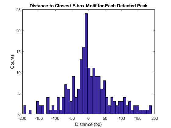
Use the knnsearch function to find the closest motif to each one of the putative peaks. As expected, most of the enriched ChIP peaks are close to an E-box motif [1]. This reinforces the importance of performing peak detection at the finest resolution possible (bp resolution) when the expected density of binding sites is high, as it is in the case of the E-box motif. This example also illustrates that for this type of analysis, paired-end sequencing should be considered over single-end sequencing [1].

h = knnsearch(motifs',putative_peaks(:,1));
distance = putative_peaks(:,1)-motifs(h(:))';
figure
histogram(distance(abs(distance)<200),50)
title('Distance to Closest E-box Motif for Each Detected Peak')
xlabel('Distance (bp)')
ylabel('Counts')

References

[1] Wang, Congmao, Jie Xu, Dasheng Zhang, Zoe A Wilson, and Dabing Zhang. “An Effective Approach for Identification of in Vivo Protein-DNA Binding Sites from Paired-End ChIP-Seq Data.” BMC Bioinformatics 11, no. 1 (2010): 81.

[2] Li, H., and R. Durbin. “Fast and Accurate Short Read Alignment with Burrows-Wheeler Transform.” Bioinformatics 25, no. 14 (July 15, 2009): 1754–60.

[3] Li, H., B. Handsaker, A. Wysoker, T. Fennell, J. Ruan, N. Homer, G. Marth, G. Abecasis, R. Durbin, and 1000 Genome Project Data Processing Subgroup. “The Sequence Alignment/Map Format and SAMtools.” Bioinformatics 25, no. 16 (August 15, 2009): 2078–79.

[4] Jothi, R., S. Cuddapah, A. Barski, K. Cui, and K. Zhao. “Genome-Wide Identification of in Vivo Protein-DNA Binding Sites from ChIP-Seq Data.” Nucleic Acids Research 36, no. 16 (August 1, 2008): 5221–31.

[5] Hoffman, Brad G, and Steven J M Jones. “Genome-Wide Identification of DNA–Protein Interactions Using Chromatin Immunoprecipitation Coupled with Flow Cell Sequencing.” Journal of Endocrinology 201, no. 1 (April 2009): 1–13.

[6] Ramsey, Stephen A., Theo A. Knijnenburg, Kathleen A. Kennedy, Daniel E. Zak, Mark Gilchrist, Elizabeth S. Gold, Carrie D. Johnson, et al. “Genome-Wide Histone Acetylation Data Improve Prediction of Mammalian Transcription Factor Binding Sites.” Bioinformatics 26, no. 17 (September 1, 2010): 2071–75.