Evaluate Performance of ACL Interframe Space in Bluetooth LE Piconet
This example shows how to simulate and evaluate the throughput and latency performance of the interframe space (IFS) types in an asynchronous connection-oriented logical (ACL) connection as specified in the Bluetooth® Core Specification v6.0 [2].
Using this example, you can:
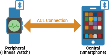
Create a Bluetooth low energy (LE) scenario consisting of a Central (smartphone) and a Peripheral (fitness watch) node.
Configure the IFS values you want to simulate and evaluate in the ACL connection between the Central and Peripheral nodes.
Add On-Off application traffic between the Bluetooth LE nodes.
Run the simulation and visualize the impact of IFS values on the throughput and latency.
Interframe Space in ACL Transport
The link layer (LL) specifies an air interface protocol, which includes defining the IFS time interval. The channel requires the IFS between any two consecutive Bluetooth LE packets transmitted upon it. Before Bluetooth Core Specification v6.0, IFS was specified by the symbolic identifier T_IFS, and had a fixed duration of 150 µs, and the same protocol also defined the minimum time duration required between the end of the last packet in an event or subevent and the beginning of the next event or subevent for various transport types.
The ACL transport enables a Bluetooth LE Central node to exchange packets with a Peripheral node during connection events. This figure shows an example of an ACL connection as specified before Bluetooth Core Specification v6.0. In this configuration, the fixed value T_IFS determines the mandatory time interval between packets within the same connection event, whether transmitted from Central to Peripheral or the other way around.
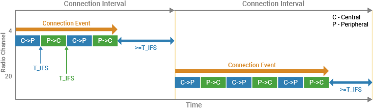
Note that a minimum interval of T_IFS also separates the end of one connection event from the start of the next.
The Bluetooth Core Specification v6.0 introduces these modifications to IFS in ACL connections:
The specification assigns three distinct symbolic names for the IFS values applicable to ACL connections.
The IFS values are no longer fixed at 150 µs.
Each of these new IFS values defaults to 150 µs. However, the Central and Peripheral nodes can negotiate new values after they establish a connection to one another.
The negotiated frame spacing values can be either shorter or longer than the default 150 µs.
This table summarizes the new IFS types for ACL connections.
IFS Type Symbolic Identifier | Description |
| The Central node must ensure this required spacing time exists between the end of a packet transmission and the start of the subsequent slot in the same connection event, which the Peripheral node might use. |
| The Peripheral node must ensure this required spacing time exists between the end of a packet transmission and the start of the subsequent slot in the same connection event, which the Central may potentially use. |
| The minimum time that must elapse between the end of one connection event and the start of the next. |
This figure shows the connection events and packet transmissions between a Central and a Peripheral node in an ACL connection, with the new IFS types represented by their symbolic identifiers.

Reducing IFS values can enhance overall data throughput and latency. Applications that benefit from shorter frame spaces and increased data rates include:
Fitness trackers — These devices can transfer accumulated data in a single batch to connected devices like smartphones or laptops.
Firmware updates — Faster data transfer speeds facilitate more efficient updates.
Bluetooth LE audio — Audio packets transmitted over a connected isochronous stream are delivered more swiftly in shorter bursts, minimizing collision risks with other devices.
Multi-purpose radios — Devices using their radio for additional functions, such as Wi-Fi®, increase the available time for these activities.
Conversely, controllers with limited processing power can benefit from longer frame space values, as they provide additional time to process longer packets.
Fitness Watch and Smartphone Scenario
The example creates, configures, and simulates a scenario consisting of a Bluetooth LE Peripheral node (fitness watch) connected to a Bluetooth LE Central node (smartphone) on an ACL transport.
The example adds On-Off application traffic between the Central and Peripheral nodes and simulates the scenario by using the configured IFS values.
Configure IFS and Initialize Performance Metrics
Specify the set of IFS values you want to simulate. The T_IFS_ACL_Values variable specifies the IFS values between the Central and Peripheral nodes. The T_MCES value specifies the minimum time that must elapse between the end of one connection event and the start of the next.
T_IFS_ACL_Values = [10 50 100 150 200 250]; % In microseconds
T_MCES = T_IFS_ACL_Values;
Initialize the throughput and latency metrics.
numTIFS = numel(T_IFS_ACL_Values);
throughput = zeros(numTIFS,1);
latency = zeros(numTIFS,1);
Create and Configure Bluetooth LE Piconet
Set the seed for the random number generator to default to ensure repeatable results. To improve the accuracy of your simulation results, after running the simulation, you can change the seed value, run the simulation again, and average the results over multiple simulations.
parfor tifsIdx = 1:numTIFS
    rng("default")
Create a wireless network simulator object. Specify the simulation time in seconds.
    networkSimulator = wirelessNetworkSimulator.init;
    simulationTime = 1;
Create a Bluetooth LE Central node and a Peripheral node, specifying their positions using x-, y-, and z-coordinates, in meters.
    centralNode = bluetoothLENode("central",Position=[0 0 0]);
    peripheralNode = bluetoothLENode("peripheral",Position=[2 0 0]);
Create a default Bluetooth LE connection configuration object.
connectionConfig = bluetoothLEConnectionConfig;
Set the IFS values, using T_IFS_ACL_Values and T_MCES. Note that this code sets the TIFS property of the connection configuration object to a scalar, which specifies the same value for T_IFS_ACL_CP and T_IFS_ACL_PC. If you want to configure distinct values for T_IFS_ACL_CP and T_IFS_ACL_PC, set the TIFS value as a vector, where the first and second elements specify the T_IFS_ACL_CP and T_IFS_ACL_PC values, respectively.
    connectionConfig.TIFS = T_IFS_ACL_Values(tifsIdx)*1e-6;  % In seconds
    connectionConfig.TMCES = T_MCES(tifsIdx)*1e-6; % In seconds
Assign the configuration to the Central and Peripheral nodes.
configureConnection(connectionConfig,centralNode,peripheralNode);
Add the Bluetooth LE nodes to the wireless network simulator.
    bluetoothLENodes = [centralNode peripheralNode];
    addNodes(networkSimulator,bluetoothLENodes)
Add Application Traffic
Create a networkTrafficOnOff object to generate an On-Off application traffic pattern. Configure the On-Off application traffic pattern at the Central and Peripheral nodes by specifying the application data rate, On state duration, Off state duration, and packet size. Add application traffic between the Central and the Peripheral nodes.
    trafficSourceC2P = networkTrafficOnOff(DataRate=1000,OnTime=Inf,OffTime=0,PacketSize=10);
    addTrafficSource(centralNode,trafficSourceC2P,DestinationNode=peripheralNode)

    trafficSourceP2C = networkTrafficOnOff(DataRate=1000,OnTime=Inf,OffTime=0,PacketSize=10);
    addTrafficSource(peripheralNode,trafficSourceP2C,DestinationNode=centralNode)
Run Simulation and Retrieve Statistics
Initialize the node performance calculation by using the helperPerformanceViewer helper object. This helper object uses the kpi object function of the bluetoothLENode object to calculate the packet loss ratio (PLR), latency, and throughput. Additionally, it stores the packet latency of each packet in a node as an array in the PacketLatency property.
performancePlotObj = helperPerformanceViewer(networkSimulator.Nodes,simulationTime);
Run the wireless network simulation for the specified simulation time.
networkSimulator.run(simulationTime)
Retrieve the statistics of all the nodes. For more information about Bluetooth LE node statistics, see the Bluetooth LE Node Statistics topic.
nodeStats = statistics(bluetoothLENodes)
Get the throughput and latency values of the network.
    throughput(tifsIdx) = sum(performancePlotObj.Throughput(:,2))
    latency(tifsIdx) = sum(performancePlotObj.AveragePacketLatency(:,2))
end
Starting parallel pool (parpool) using the 'Processes' profile ...
Connected to parallel pool with 4 workers.
Simulation Results
Plot the throughput and latency corresponding to each configured IFS value. Observe that the smaller IFS values provide higher throughput and lower latency performance. A smaller IFS enables a channel to transmit more packets compared to a larger IFS, resulting in increased throughput. Conversely, greater spacing between packets reduces the number of packets that a connection event can accommodate. Because a smaller IFS accommodates more packets, enabling faster transmission and reception when a significant amount of data is generated simultaneously, it also reduces latency.
figure
subplot(2,1,1)
plot(1:numTIFS,throughput,Marker="square",LineWidth=2,MarkerSize=5)
fontsize(gca,10,"points")
xticks(1:numTIFS)
xticklabels(string(T_IFS_ACL_Values))
xlabel("IFS (in microseconds)")
ylabel("Throughput (in Mbps)")
title("Average Throughput")
subplot(2,1,2)
plot(1:numTIFS,latency,Marker="*",LineWidth=2,MarkerSize=5)
fontsize(gca,10,"points")
xticklabels(string(T_IFS_ACL_Values))
xlabel("IFS (in microseconds)")
ylabel("Latency (in seconds)")
title("Average APP Latency")

Appendix
The example uses this helper object.
helperPerformanceViewer — Return a performance metrics viewer object.
References
1] Bluetooth Technology Website. "Bluetooth Technology Website | The Official Website of Bluetooth Technology". Accessed December 01, 2024. https://www.bluetooth.com/.
[2] Bluetooth Core Specifications Working Group. "Bluetooth Core Specification" v6.0. Accessed December 01, 2024. https://www.bluetooth.com/specifications/specs/core-specification-6-0/.