sigstrength

Received signal strength

collapse all in page

Syntax

ss = sigstrength(rx,tx)

ss = sigstrength(rx,tx,propmodel)

ss = sigstrength(___,Name=Value)

Description

ss = sigstrength(rx,tx) returns the signal strength at the receiver site due to the transmitter site.

example

ss = sigstrength(rx,tx,propmodel) returns the signal strength at the receiver site using the specified propagation model. Specifying a propagation model is the same as specifying the PropagationModel name-value argument.

ss = sigstrength(___,Name=Value) specifies options using name-value arguments, in addition to any combination of arguments from the previous syntaxes. For example, Type="efield" returns the signal strength in electric field strength units (dBμV/m).

Examples

collapse all

Received Power and Link Margin at Receiver

Open Live Script

Create a transmitter site.

tx = txsite(Name="Fenway Park", ...
    Latitude=42.3467, ...
    Longitude=-71.0972);

Create a receiver site with sensitivity defined in dBm.

 rx = rxsite(Name="Bunker Hill Monument", ...
     Latitude=42.3763, ...
     Longitude=-71.0611, ...
     ReceiverSensitivity=-90);

Calculate the received power and link margin. Link margin is the difference between the receiver's sensitivity and the received power.

ss = sigstrength(rx,tx)

ss = -71.1414

margin = abs(rx.ReceiverSensitivity - ss)

margin = 18.8586

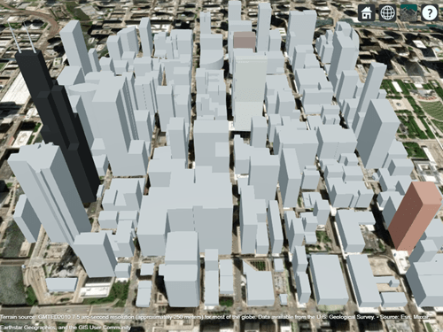
Signal Strength Using Ray Tracing Propagation Model

Open Live Script

Launch Site Viewer with buildings in Chicago. For more information about the OpenStreetMap® file, see [1].

viewer = siteviewer(Buildings="chicago.osm");

Site Viewer with buildings

Create a transmitter site on a building.

tx = txsite(Latitude=41.8800, ...
    Longitude=-87.6295, ...
    TransmitterFrequency=2.5e9);

Create a receiver site near another building.

rx = rxsite(Latitude=41.881352, ...
    Longitude=-87.629771, ...
    AntennaHeight=30);

Create a ray tracing propagation model, which MATLAB® represents using a RayTracing object. By default, the propagation model uses the SBR method and finds propagation paths with up to two surface reflections.

pm = propagationModel("raytracing");

Calculate the signal strength using the receiver site, the transmitter site, and the propagation model.

ssTwoReflections = sigstrength(rx,tx,pm)

ssTwoReflections = -54.3151

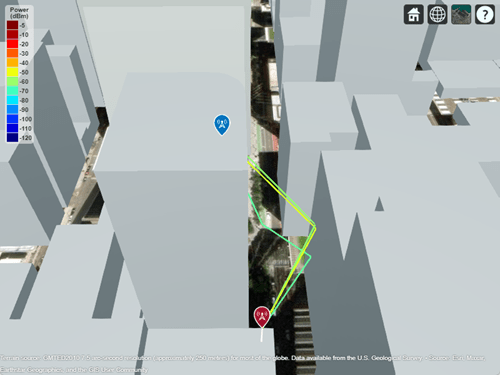
Plot the propagation paths.

raytrace(tx,rx,pm)

Three propagation paths from the transmitter site to the receiver site

Change the RayTracing object to find paths with up to 5 reflections. Then, recalculate the signal strength.

pm.MaxNumReflections = 5;
ssFiveReflections = sigstrength(rx,tx,pm)

ssFiveReflections = -53.3965

By default, RayTracing objects use concrete terrain materials and building materials derived from the OpenStreetMap file. When the OpenStreetMap file does not specify materials, the model uses concrete. Change the building and terrain material types to model perfect electrical conductors.

pm.TerrainMaterial = "perfect-reflector";
pm.BuildingsMaterial = "perfect-reflector";

ssPerfect = sigstrength(rx,tx,pm)

ssPerfect = -38.9334

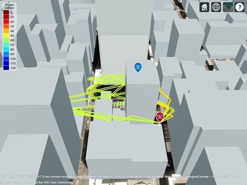
Plot the propagation paths for the updated propagation model.

raytrace(tx,rx,pm)

Additional propagation paths from the transmitter site to the receiver site

Appendix

[1] The OpenStreetMap file is downloaded from https://www.openstreetmap.org, which provides access to crowd-sourced map data all over the world. The data is licensed under the Open Data Commons Open Database License (ODbL), https://opendatacommons.org/licenses/odbl/.

Input Arguments

collapse all

`rx` — Receiver site
`rxsite` object | array of `rxsite` objects

Receiver site, specified as an rxsite object or an array of rxsite objects.

`tx` — Transmitter site
`txsite` object | array of `txsite` objects

Transmitter site, specified as a txsite object or an array of txsite objects.

`propmodel` — Propagation model to use for path loss calculations
`"longley-rice"` (default) | `"freespace"` | `"close-in"` | `"rain"` | `"gas"` | `"fog"` | `"raytracing"` | propagation model created using `propagationModel`

Propagation model to use for the path loss calculations, specified as one of these options:

"freespace" — Free space propagation model
"rain" — Rain propagation model
"gas" — Gas propagation model
"fog" — Fog propagation model
"close-in" — Close-in propagation model
"longley-rice" — Longley-Rice propagation model
"tirem" — TIREM™ propagation model
"raytracing" — Ray tracing propagation model that uses the shooting and bouncing rays (SBR) method. When you specify a ray tracing model as input, the function incorporates multipath interference by using a phasor sum.
A propagation model created using the propagationModel function. For example, you can create a ray tracing propagation model that uses the image method by specifying propagationModel("raytracing","Method","image").

The default value depends on the coordinate system used by the input sites.

Coordinate System	Default propagation model value
`"geographic"`	`"longley-rice"` when you use a terrain. `"freespace"` when you do not use a terrain.
`"cartesian"`	`"freespace"` when `Map` is set to none. `"raytracing"` when `Map` is set to the name of a glTF™ file, the name of an STL file, or a triangulation object. The default ray tracing model uses the shooting and bouncing rays (SBR) method.

Terrain propagation models, including "longley-rice" and "tirem", are only supported for sites with a CoordinateSystem value of "geographic".

You can also specify the propagation model by using the PropagationModel name-value pair argument.

Name-Value Arguments

Specify optional pairs of arguments as Name1=Value1,...,NameN=ValueN, where Name is the argument name and Value is the corresponding value. Name-value arguments must appear after other arguments, but the order of the pairs does not matter.

Example: sigstrength(rx,tx,Type="efield") returns the signal strength in electric field strength units (dBμV/m).

Before R2021a, use commas to separate each name and value, and enclose Name in quotes.

Example: sigstrength(rx,tx,"Type","efield") returns the signal strength in electric field strength units (dBμV/m).

`Type` — Type of signal strength to compute
`"power"` (default) | `"efield"`

Type of signal strength to compute, specified as one of these options:

"power" — The signal strength is in power units (dBm) of the signal at the mobile receiver input.
"efield"— The signal strength is in electric field strength units (dBμV/m) of signal wave incident on the antenna.

Data Types: char | string

`PropagationModel` — Propagation model to use for path loss calculations
`"freespace"` | `"close-in"` | `"rain"` | `"gas"` | `"fog"` | `"longley-rice"` | `"raytracing"` | propagation model created using `propagationModel`

Propagation model to use for the path loss calculations, specified as one of these options:

"freespace" — Free space propagation model
"rain" — Rain propagation model
"gas" — Gas propagation model
"fog" — Fog propagation model
"close-in" — Close-in propagation model
"longley-rice" — Longley-Rice propagation model
"tirem" — TIREM propagation model
"raytracing" — Ray tracing propagation model that uses the shooting and bouncing rays (SBR) method. When you specify a ray tracing model as input, the function incorporates multipath interference by using a phasor sum.
A propagation model created using the propagationModel function. For example, you can create a ray tracing propagation model that uses the image method by specifying propagationModel("raytracing","Method","image").

The default value depends on the coordinate system used by the input sites.

Coordinate System	Default propagation model value
`"geographic"`	`"longley-rice"` when you use a terrain. `"freespace"` when you do not use a terrain.
`"cartesian"`	`"freespace"` when `Map` is set to none. `"raytracing"` when `Map` is set to the name of a glTF file, the name of an STL file, or a triangulation object. The default ray tracing model uses the shooting and bouncing rays (SBR) method.

Terrain propagation models, including "longley-rice" and "tirem", are only supported for sites with a CoordinateSystem value of "geographic".

Data Types: char | string

`Map` — Map for visualization or surface data
`siteviewer` object | `triangulation` object | string scalar | character vector

Map for visualization or surface data, specified as a siteviewer object, a triangulation object, a string scalar, or a character vector. Valid and default values depend on the coordinate system.

Coordinate System	Valid map values	Default map value
`"geographic"`	A `siteviewer` object^a A terrain name, if the function is called with an output argument. Valid terrain names are `"none"`, `"gmted2010"`, or the name of the custom terrain data added using `addCustomTerrain`.	The current `siteviewer` object or a new `siteviewer` object if none are open `"gmted2010"`, if the function is called with an output
`"cartesian"`	`"none"` A `siteviewer` object The name of a glTF file The name of an STL file A `triangulation` object	`"none"`
^a Alignment of boundaries and region labels are a presentation of the feature provided by the data vendors and do not imply endorsement by MathWorks^®.

In most cases, if you specify this argument as a value other than a siteviewer or "none", then you must also specify an output argument.

Data Types: char | string

Output Arguments

collapse all

`ss` — Signal strength
M-by-N array

Signal strength, returned as M-by-N array, where M is the number of transmitter sites and N is the number of receiver sites.

The units of ss depend on the value of the Type name-value argument.

When you specify Type as "power", then ss is in power units (dBm) of the signal at the mobile receiver input.
When you specify Type as "efield", then ss is in electric field strength units (dBμV/m) of signal wave incident on the antenna.

References

[1] International Telecommunications Union Radiocommunication Sector. Effects of Building Materials and Structures on Radiowave Propagation Above About 100MHz. Recommendation P.2040. ITU-R, approved August 23, 2023. https://www.itu.int/rec/R-REC-P.2040/en.

[2] International Telecommunications Union Radiocommunication Sector. Electrical Characteristics of the Surface of the Earth. Recommendation P.527. ITU-R, approved September 27, 2021. https://www.itu.int/rec/R-REC-P.527/en.

Version History

Introduced in R2019b

expand all

R2024a: Ray tracing functions model materials using updated ITU recommendations

When calculating received power using ray tracing models, the sigstrength function models materials using the methods and equations in International Telecommunication Union Recommendations (ITU-R) P.2040-3 [1] and ITU-R P.527-5 through ITU-R P.527-6 [2].

In previous releases, the function used ITU-R P.2040-1. As a result of these changes, the sigstrength function can return different values in R2024a compared to previous releases.

R2023b: Perform ray tracing analysis with multiple materials in the same scene

The sigstrength function performs ray tracing analysis with multiple materials in the same scene when:

You create the scene from a glTF file, and specify the propmodel input argument as "raytracing" or a RayTracing propagation model object with its SurfaceMaterial property set to "auto" (the default).
You create the scene from an OpenStreetMap^® file or a geospatial table, and you specify the propmodel input argument as "raytracing" or a RayTracing propagation model object with its BuildingsMaterial property set to "auto" (the default).

The sigstrength function performs the ray tracing analysis using the materials stored in the file or table. If the file or table does not specify materials, or if the file or table specifies a material that the ray tracing analysis does not support, then the function uses concrete instead of the absent or unsupported material.

As a result, the sigstrength function can return different values in R2023b compared to previous releases. To avoid using the materials stored in the file or table, create a RayTracing object (by using the propagationModel function) and set its SurfaceMaterial property to "plasterboard" and its BuildingsMaterial property to "concrete". Then, use the object as input to the sigstrength function.

R2023b: Ray tracing analysis with SBR method shows improved performance in complex scenes

The sigstrength function shows improved performance with complex scenes when you specify a RayTracing propagation model object that uses the shooting and bouncing rays (SBR) method as input.

The time that MATLAB^® requires to perform ray tracing analysis depends on the scene and on the properties of the RayTracing object, such as the AngularSeparation, MaxNumDiffractions, MaxNumReflections, MaxAbsolutePathLoss, and MaxRelativePathLoss properties. In some cases, with moderate values of the MaxAbsolutePathLoss and MaxRelativePathLoss properties, the ray tracing analysis can be more than 2x faster in R2023b than in R2023a.

R2023a: Ray tracing models discard paths based on path loss

Ray tracing propagation models discard propagation paths based on path loss thresholds. By default, when you specify the propmodel input argument as "raytracing" or a RayTracing object, the propagation model discards paths that are more than 40 dB weaker than the strongest path.

As a result, the sigstrength function can return different values in R2023a compared to previous releases. To avoid discarding paths based on relative path loss thresholds, create a RayTracing object (by using the propagationModel function) and set its MaxRelativePathLoss property to Inf. Then, use the object as input to the sigstrength function.

R2022b: Ray tracing functions consider multipath interference

When calculating received power using ray tracing models, the sigstrength function now considers multipath interference by using a phasor sum. In previous releases, the function used a power sum. As a result, the calculations in R2022b are more accurate than in previous releases.

R2021b: `"raytracing"` propagation models use SBR method

Starting in R2021b, when you use the sigstrength function and specify the propmodel argument or PropagationModel name-value argument as "raytracing", the function uses the shooting and bouncing rays (SBR) method and calculates up to two reflections. In previous releases, the sigstrength function uses the image method and calculates up to one reflection.

To calculate received signal strength using the image method instead, create a propagation model by using the propagationModel function. Then, use the sigstrength function with the propagation model as input. This example shows how to update your code.

pm = propagationModel("raytracing","Method","image");
ss = sigstrength(rx,tx,pm)

For information about the SBR and image methods, see Choose a Propagation Model.

Starting in R2021b, all RF Propagation functions use the SBR method by default and calculate up to two reflections. For more information, see Default modeling method is shooting and bouncing rays method.

sigstrength

Syntax

Description

Examples

Received Power and Link Margin at Receiver

Signal Strength Using Ray Tracing Propagation Model

Input Arguments

`rx` — Receiver site
`rxsite` object | array of `rxsite` objects

`tx` — Transmitter site
`txsite` object | array of `txsite` objects

`propmodel` — Propagation model to use for path loss calculations
`"longley-rice"` (default) | `"freespace"` | `"close-in"` | `"rain"` | `"gas"` | `"fog"` | `"raytracing"` | propagation model created using `propagationModel`

Name-Value Arguments

`Type` — Type of signal strength to compute
`"power"` (default) | `"efield"`

`PropagationModel` — Propagation model to use for path loss calculations
`"freespace"` | `"close-in"` | `"rain"` | `"gas"` | `"fog"` | `"longley-rice"` | `"raytracing"` | propagation model created using `propagationModel`

`Map` — Map for visualization or surface data
`siteviewer` object | `triangulation` object | string scalar | character vector

Output Arguments

`ss` — Signal strength
M-by-N array

References

Version History

R2024a: Ray tracing functions model materials using updated ITU recommendations

R2023b: Perform ray tracing analysis with multiple materials in the same scene

R2023b: Ray tracing analysis with SBR method shows improved performance in complex scenes

R2023a: Ray tracing models discard paths based on path loss

R2022b: Ray tracing functions consider multipath interference

R2021b: `"raytracing"` propagation models use SBR method

See Also

Functions

sigstrength

Syntax

Description

Examples

Received Power and Link Margin at Receiver

Signal Strength Using Ray Tracing Propagation Model

Input Arguments

rx — Receiver site rxsite object | array of rxsite objects

tx — Transmitter site txsite object | array of txsite objects

propmodel — Propagation model to use for path loss calculations "longley-rice" (default) | "freespace" | "close-in" | "rain" | "gas" | "fog" | "raytracing" | propagation model created using propagationModel

Name-Value Arguments

Type — Type of signal strength to compute "power" (default) | "efield"

PropagationModel — Propagation model to use for path loss calculations "freespace" | "close-in" | "rain" | "gas" | "fog" | "longley-rice" | "raytracing" | propagation model created using propagationModel

Map — Map for visualization or surface data siteviewer object | triangulation object | string scalar | character vector

Output Arguments

ss — Signal strength M-by-N array

References

Version History

R2024a: Ray tracing functions model materials using updated ITU recommendations

R2023b: Perform ray tracing analysis with multiple materials in the same scene

R2023b: Ray tracing analysis with SBR method shows improved performance in complex scenes

R2023a: Ray tracing models discard paths based on path loss

R2022b: Ray tracing functions consider multipath interference

R2021b: "raytracing" propagation models use SBR method

See Also

Functions

`rx` — Receiver site
`rxsite` object | array of `rxsite` objects

`tx` — Transmitter site
`txsite` object | array of `txsite` objects

`propmodel` — Propagation model to use for path loss calculations
`"longley-rice"` (default) | `"freespace"` | `"close-in"` | `"rain"` | `"gas"` | `"fog"` | `"raytracing"` | propagation model created using `propagationModel`

`Type` — Type of signal strength to compute
`"power"` (default) | `"efield"`

`PropagationModel` — Propagation model to use for path loss calculations
`"freespace"` | `"close-in"` | `"rain"` | `"gas"` | `"fog"` | `"longley-rice"` | `"raytracing"` | propagation model created using `propagationModel`

`Map` — Map for visualization or surface data
`siteviewer` object | `triangulation` object | string scalar | character vector

`ss` — Signal strength
M-by-N array

R2021b: `"raytracing"` propagation models use SBR method