Cosine Similarity As a Channel Estimate Quality Metric

Generic Cosine Similarity for Matrices

Given an $$mx$$-by-$$n$$ data matrix $$X$$, which is treated as $$mx$$ (1-by-$$n$$) row vectors $$x_1$$, $$x_2$$, ..., $$x_{mx}$$, and an $$my$$-by-$$n$$ data matrix $$Y$$, which is treated as $$my$$ (1-by-$$n$$) row vectors $$y_1$$, $$y_2$$, ..., $$y_{my}$$, the cosine similarity between the vector $$x_p$$ and $$y_q$$ are defined as follows:

$$s=\frac{x_p^H.y_q}{\sqrt{(x_p^H.x_p)(y_q^H.y_q)}}$$.

The helperComplexCosineSimilarity function calculates the cosine similarity between the $$p^{th}$$ row of $$X$$ and $$q^{th}$$ row of $$Y$$. Create the matrix $$X$$ as a random complex-valued matrix.

rng(123) % Generate same numbers
X = randn(4,3,"like",1i)

X = 4×3 complex

   0.5404 - 0.4278i  -0.0233 - 0.2087i  -0.6441 - 0.3274i
  -0.7318 + 0.1424i  -0.3923 + 0.3991i   0.0868 + 0.0637i
   0.4723 - 0.2287i  -0.0946 - 1.1849i   0.2262 + 0.7520i
   0.9435 + 0.4394i  -0.2465 + 0.5979i   0.6372 + 0.2031i

The $$Y$$ matrix is the noisy version of $$X$$.

Y = awgn(X,10)

Y = 4×3 complex

   0.6792 - 0.5721i  -0.0525 - 0.2112i  -0.5521 - 0.5331i
  -0.8135 + 0.0120i  -0.4151 + 0.1926i  -0.0387 - 0.0079i
   0.1660 - 0.1073i  -0.1616 - 0.8501i   0.6504 + 0.6647i
   0.5617 + 0.4250i   0.0638 + 0.5991i   0.6256 + 0.4346i

The helperComplexCosineSimilarity function calculates the cosine similarity between rows of two arrays. When the operation method is "perm", the function calculates the similarity for all permutations of rows. Since $$y_p$$ is the noisy version of $$x_p$$, the diagonal similarity values are close to 1. Since the rows of X are independent, the off-diagonal values are smaller.

cosimperm = helperComplexCosineSimilarity(X,Y,"perm")

cosimperm = 4×4 complex

   0.9747 + 0.1133i  -0.6464 + 0.3702i   0.0999 + 0.0759i  -0.1104 - 0.5895i
  -0.4697 - 0.4618i   0.9500 + 0.2270i  -0.4164 - 0.4676i  -0.4378 + 0.4388i
  -0.2438 - 0.1647i  -0.2602 + 0.3889i   0.9081 - 0.2370i   0.1061 + 0.2359i
  -0.4492 + 0.3220i  -0.0484 - 0.5806i  -0.0437 - 0.0132i   0.9231 + 0.0705i

Cosine Similarity for CSI

When $$X$$ is a channel matrix, only the similarity between the $$p^{th}$$ row of $$X$$ and $$p^{th}$$ row $$Y$$ are important. Call the helperComplexCosineSimilarity function with the "rows" option.

cosimrows = helperComplexCosineSimilarity(X,Y,"rows")

cosimrows = 4×1 complex

   0.9747 + 0.1133i
   0.9500 + 0.2270i
   0.9081 - 0.2370i
   0.9231 + 0.0705i

Calling the function with the "meanrows" option calculates the mean of cosine similarity of all the corresponding rows, which is calculated using the "rows" option. The "meanrows" operation method is the default value.

cosimmean = helperComplexCosineSimilarity(X,Y)

cosimmean = 
0.9390 + 0.0434i

Test With Compressed and Decompressed CSI

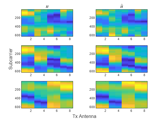
Load the original channel estimate, $$H$$, and the compressed and decompressed channel estimate, $$\underset{}{\overset{ˆ}{H}}$$, obtained using 4-bit quantization in the CSI Feedback with Autoencoders example. The dimensions of $$H$$ are subcarriers, transmit antennas, and realizations. The $$H$$ and $$\underset{}{\overset{ˆ}{H}}$$ pairs have –0.78 dB, –6.4 dB, –12.5 dB NMSE for the three realizations in this example.

load csi_cosim_test_data.mat H Hhat
t=tiledlayout(3,2);
ylabel(t,"Subcarrier")
xlabel(t,"Tx Antenna")
nexttile
imagesc(abs(H(:,:,1)))
title("$H$",Interpreter="latex")
nexttile
imagesc(abs(Hhat(:,:,1)))
title("$\hat{H}$",Interpreter="latex")
nexttile
imagesc(abs(H(:,:,2)))
nexttile
imagesc(abs(Hhat(:,:,2)))
nexttile
imagesc(abs(H(:,:,3)))
nexttile
imagesc(abs(Hhat(:,:,3)))

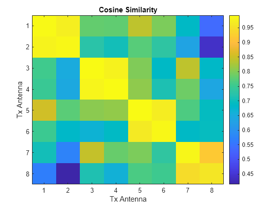
Run the cosine similarity along the subcarriers for each of the eight antennas. Since $$H$$ and $$\underset{}{\overset{ˆ}{H}}$$ store subcarriers in the first dimension, transpose the matrices to place subcarriers in the rows (second dimension). Off-diagonal values show the similarity between different antennas and have lower values. The helperComplexCosineSimilarity function processes all three realizations at the same time by using batch processing, where the third dimension is the batch (page) dimension. The pagectranspose function applies the complex conjugate transpose to each page of $$H$$ and $$\underset{}{\overset{ˆ}{H}}$$.

cosimperm = helperComplexCosineSimilarity(pagectranspose(H),pagectranspose(Hhat),"perm");

Select the index of the batch to examine.

idx = 1;
figure
imagesc(abs(cosimperm(:,:,idx)))
xlabel("Tx Antenna")
ylabel("Tx Antenna")
title("Cosine Similarity")
colorbar

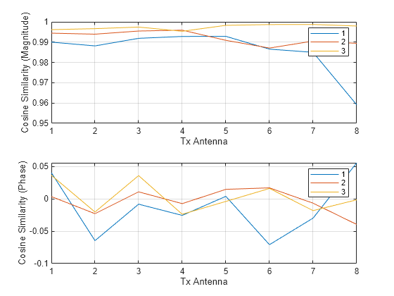
Plot the cosine similarity between the same antennas.

cosimrows = helperComplexCosineSimilarity(pagetranspose(H),pagetranspose(Hhat),"rows");
subplot(2,1,1)
plot(abs(squeeze(cosimrows)))
grid on
xlabel("Tx Antenna")
ylabel("Cosine Similarity (Magnitude)")
legend("1","2","3")
subplot(2,1,2)
plot(angle(squeeze(cosimrows)))
grid on
xlabel("Tx Antenna")
ylabel("Cosine Similarity (Phase)")
legend("1","2","3")

Calculate cosine similarity across all Tx antennas.

cosimmean = helperComplexCosineSimilarity(pagetranspose(H),pagetranspose(Hhat))

cosimmean = 
cosimmean(:,:,1) =

   0.9848 - 0.0123i


cosimmean(:,:,2) =

   0.9920 - 0.0037i


cosimmean(:,:,3) =

   0.9971 + 0.0026i