OFDM Transmitter and Receiver
This example shows how to run a complete link-level OFDM transmission system for a single-input single-output (SISO) channel. The physical-layer transmission protocol mimics typical synchronization signals, reference symbols, control channels, and data channels popular across standardized transmission schemes such as LTE, 5G NR, and WLAN. The example can be used to test different transmission signals and receiver algorithms across various channels and radio impairments. This processing includes scrambling, convolutional encoding, modulation, filtering, channel distortion, demodulation, maximum likelihood decoding, and more.
The transmitter models control channels and data channels in this example. Transmitted data bits are split into transport blocks and OFDM-modulated. Control signals are multiplexed in with the data signals for synchronization, signaling, and estimation of impairments. Channel impairments distort the transmitted signal in the time domain. The impairments include multipath fading and noise, and carrier frequency offset is modeled as a receiver impairment. The receiver models sample buffering for timing adjustment, filtering, carrier frequency adjustment, and OFDM demodulation and decoding.
The example allows exploration of different system parameters, channel impairments, and receiver operations through editor controls. Visualization aids are also enabled or disabled through editor controls to see the effects of the different combinations of parameters, impairments, and receiver algorithms.
System Parameters
Select the system parameters from a set of allowed values. These parameters are transmitted within the frame header and decoded by the receiver. The entries are representative of typical LTE, WLAN, and 5G NR transmission parameters. More entries may be added as desired, taking note that most parameters have interdependencies on other parameters.
BWIndex = {FFT length, CP length, number of occupied subcarriers, subcarrier spacing, pilot subcarrier spacing, channel BW}:
1 = {128, 32, 72, 15e3, 9, 1.4e6}
2 = {256, 64, 180, 15e3, 20, 3e6}
3 = {512, 128, 300, 15e3, 20, 5e6}
4 = {1024, 256, 600, 15e3, 20, 10e6} (default)
5 = {2048, 512, 1200, 15e3, 24, 20e6}
6 = {128, 32, 112, 312.5e3, 14, 35.6e6}
7 = {4096, 1024, 3276, 30e3, 36, 98.28e6}
Modulation order for all data subcarriers:
2 = BPSK
4 = QPSK
16 = 16-QAM
64 = 64-QAM (default)
256 = 256-QAM
1024 = 1024-QAM
Code rate:
0 = 1/2 (default)
1 = 2/3
2 = 3/4
3 = 5/6
Several controls are available to enable or disable receiver impairments and scopes for transceiver visualization. It is recommended that visualizations be disabled for long simulations and/or simulations over multiple SNRs. Controls are also available to enable or disable certain receiver algorithms.
Change the output verbosity to control the diagnostic output text. The "Low" setting suppresses diagnostic output during frame processing. The "High" setting enables all output.
% Clear persistent state variables and buffers, and close all figures clear helperOFDMRx helperOFDMRxFrontEnd helperOFDMRxSearch helperOFDMChannel helperOFDMFrequencyOffset close all; userParam = struct( ... 'BWIndex',4, ... % Index corresponding to desired bandwidth 'modOrder',
64, ... % Subcarrier constellation modulation order 'codeRateIndex',
0, ... % Code rate index corresponding to desired rate 'numSymPerFrame',
15, ... % Number of OFDM symbols per frame 'numFrames',
100, ... % Number of frames to be generated for simulation (12-500) 'fc',
1900000000, ... % Carrier frequency (Hz) 'enableFading',
true , ... % Enable/disable channel fading 'chanVisual',
"Off", ... % Channel fading visualization option 'enableCFO',
true , ... % Enable/disable carrier frequency offset compensation 'enableCPE',
true , ... % Enable/disable common phase error compensation 'enableScopes',
true , ... % Enable/disable scopes 'verbosity',
0); % Diagnostic output verbosity
Mobile Environment and Impairments
Specify the impairments and the desired signal-to-noise ratio (SNR) assuming no channel loss or fading. Specify the SNR as a scalar value or create a vector of SNR values to run multiple simulations at different SNRs, and then create a BER plot. Note that sync symbol detection at low SNRs may not be possible.
The velocity inversely affects the channel coherence time (specifically, the amount of time the channel distortion is roughly constant). Since the beginning of each frame contains a reference signal to measure the channel distortion, set the velocity so that the coherence time is sufficiently greater than the frame period (controlled by the number of symbols per frame). To select a velocity, consider a generally accepted estimate of the coherence time , where is the speed of light, is the velocity, and is the carrier frequency.
The frequency offset is the difference between the transmitter and receiver at the baseband frequency. This parameter is commonly expressed in parts per million (ppm). For example, a 100 Hz offset with respect to a sampling frequency of 30.72 MHz yields an offset of 3.25 ppm.
The fading path delays and gains control the number of paths and average gain in dB of each path. A scalar entry for each constitutes a flat fading channel, and a vector specifies multi-path fading. You can see the effects of flat vs. multi-path fading by enabling the scopes and comparing the spectrum plots. Multipath fading causes nulls in some parts of the transmitted spectrum; interleaving helps to spread user data across all frequencies, so that some of the redundant bits are received on unaffected subcarriers. Decreasing the coding rate in the system parameters also helps to generate more redundant bits and increase the chances of error correction, but at the cost of lower user data throughput.
SNRdB =20:5:30; % SNR in dB v =
40; % mobile velocity (km/h) foff =
3.25; % frequency offset (ppm) fadingPathDelays =
[0 0.1e-6 0.3e-6]; fadingPathGains =
[0 1 -9]; BERResults = zeros(size(SNRdB));
Populate Parameter Structure
The helper function helperOFDMSetParameters configures the system parameters common to the transmitter and receiver.
Coding parameters specify the channel coding parameters that are applied to the data payload for scrambling, interleaving, and convolutional encoding purposes. These parameters are shared between the transmitter and receiver. The system uses a 7th-degree scrambler polynomial, interleaving depth of 12 for header data and 18 for payload data, a base convolutional coding rate of 1/2, and a 32-bit CRC.
[sysParam, txParam] = helperOFDMSetParameters(userParam);

[~,codeParam] = helperOFDMGetTables(userParam.BWIndex,userParam.codeRateIndex);
codeRate = codeParam.codeRate; % Coding rate

fprintf('\nTransmitting at %d MHz with an occupied bandwidth of %d MHz\n', ...
    sysParam.fc/1e6,sysParam.scs*sysParam.usedSubCarr/1e6);
Transmitting at 1900 MHz with an occupied bandwidth of 9 MHz
% Calculate fading channel impairments
KPH_TO_MPS = (1000/3600);
fsamp = sysParam.scs*sysParam.FFTLen;       % sample rate of signal
T = (sysParam.FFTLen+sysParam.CPLen)/fsamp; % symbol duration (s)
fmax = v * KPH_TO_MPS * sysParam.fc / physconst('LightSpeed');  % Maximum Doppler shift of diffuse components (Hz)

% Set up scopes
if userParam.enableScopes
    % Set up constellation diagram object
    refConstHeader = qammod(0:1,2,UnitAveragePower=true); % header is always BPSK
    refConstData   = qammod(0:txParam.modOrder-1,txParam.modOrder,UnitAveragePower=true);
    constDiag = comm.ConstellationDiagram(2, ...
        "ChannelNames",{'Header','Data'}, ...
        "ReferenceConstellation",{refConstHeader,refConstData}, ...
        "ShowLegend",true, ...
        "EnableMeasurements",true);

    % Set up spectrum analyzer visualization object
    sa = spectrumAnalyzer( ...
        'Name',             'Signal Spectra', ...
        'Title',            'Transmitted and Received Signal', ...
        'SpectrumType',     'Power', ...
        'FrequencySpan',    'Full', ...
        'SampleRate',       fsamp, ...
        'ShowLegend',       true, ...
        'Position',         [200 300 700 500], ...
        'ChannelNames',     {'Transmitted','Received'});
end
Initialize States and Process Data Frames
For each SNR specified in the user settings, the receiver begins in an unsynchronized, unassociated, and unconnected state. The receiver must detect the start of a frame through sync symbol detection and synchronize the receive sample buffers to begin storing samples when the beginning of the transmit frame is received. The receiver must then estimate the frequency offset and align its internal clock to match the transmitter clock; it is then considered "camped" (associated) with the base station. Finally, after header information is received and decoded, the receiver transitions to a connected state and begins decoding data.
Once connected, the simulation loops though the frame processing to generate a transmit frame, distort the output samples through a channel filter, and process the received samples to produce the transport block bitstream.
% Initialize transmitter
txObj = helperOFDMTxInit(sysParam);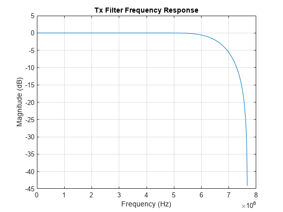
% Initialize receiver
rxObj = helperOFDMRxInit(sysParam);

for simLoopIdx = 1:length(SNRdB)
    % Configure the channel
    chanParam = struct( ...
        'SNR',       SNRdB(simLoopIdx), ...
        'foff',      foff, ...       % normalized frequency offset (ppm)
        'doppler',   fmax*T, ...     % normalized Doppler frequency
        'pathDelay', fadingPathDelays, ...
        'pathGain',  fadingPathGains);
    fprintf('Configuring the fading AWGN channel at %d dB SNR and %d kph...\n', SNRdB(simLoopIdx), v);

    sysParam.txDataBits = []; % clear tx data buffer

    sysParam.timingAdvance = (sysParam.FFTLen + sysParam.CPLen) * ...
        sysParam.numSymPerFrame; % set sample buffer timing advance

    % Instantiate an ErrorRate object to cumulatively track BER
    errorRate = comm.ErrorRate();

    fprintf('Transmitting %d frames with transport block size of %d bits per frame...\n', ...
        sysParam.numFrames,sysParam.trBlkSize);
    fprintf('Searching for synchronization symbol...');

    % Loop through all frames. Generate one extra frame to obtain the
    % reference symbol for channel estimates of the last frame.
    for frameNum = 1:sysParam.numFrames+1
        sysParam.frameNum = frameNum;
Configuring the fading AWGN channel at 20 dB SNR and 40 kph...
Transmitting 100 frames with transport block size of 20482 bits per frame...
Searching for synchronization symbol...
Configuring the fading AWGN channel at 25 dB SNR and 40 kph...
Transmitting 100 frames with transport block size of 20482 bits per frame...
Searching for synchronization symbol...
Configuring the fading AWGN channel at 30 dB SNR and 40 kph...
Transmitting 100 frames with transport block size of 20482 bits per frame...
Searching for synchronization symbol...
Payload Generation
User data is packed into a transport block, which is transmitted once per frame. The size of the transport block depends on the number of active subcarriers, number of pilot subcarriers that occupy active subcarriers, modulation order, coding rate, CRC length, encoder constraint length, and number of data symbols per frame.
Randomly generated data is used to pack the transport blocks, but custom data can be sent if desired. The data must be split into transport blocks, with the last block padded with zeros if necessary.
        % Generate random data to transmit. Replace with user data if desired.
        txParam.txDataBits  = randi([0 1],sysParam.trBlkSize,1);

        % Store data bits for BER calculations
        sysParam.txDataBits = [sysParam.txDataBits; txParam.txDataBits];
        sysParam.txDataBits = sysParam.txDataBits(max(1,end-2*sysParam.trBlkSize):end);
Transmitter Processing
The transmission grid populates signals and channels on a per-frame basis. The figure below shows one transmission frame of 24 OFDM symbols with FFT length of 256.
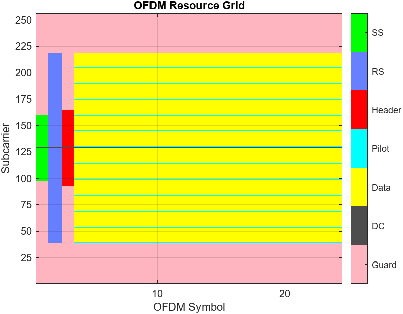
Synchronization Symbol (SS)
A synchronization (sync) signal is transmitted as the first symbol in the frame and consists of a 62-subcarrier signal centered at DC. This signal is designed to be bandwidth agnostic, meaning that all transmitters can transmit this signal regardless of the allocated bandwidth for that cell. The signal is meant to be detected by receivers to positively detect the cell signal and identify the frame boundary (the start of the frame).
Reference Symbol (RS)
A reference symbol is transmitted next. The reference symbol provides the receiver with a known reference to measure the channel distortion between the transmitter and receiver. The receiver processing can compensate for that distortion to recover the original signal as much as possible.
Header Symbol
The header conveys the bandwidth, subcarrier modulation scheme, and code rate of the OFDM data symbols to the receiver so that the receiver can properly decode the remainder of the frame. The information is important enough that it is transmitted with large signaling and coding margins to maximize correct decoding. Therefore, the symbol is coded at 1/2 rate with wide interleaving and modulated using BPSK. Since the channel distortion may change over time, the header symbol is transmitted immediately after the reference symbol to maximize the probability of correct reception. Because the bandwidth is not yet known, the header is always transmitted with a 72-subcarrier signal centered at DC.
Pilot Signals
Finally, to combat phase jitter seen at higher transmission frequencies, a pilot is transmitted at fixed subcarrier intervals within the data symbols to provide a phase reference to the receiver.
DC and Guard Subcarriers
Null subcarriers at the edge of the transmission spectrum are used to constrain spectral energy to a specified bandwidth. The subcarrier at DC is also nulled to keep the signal energy to within the linear range of the power amplifier.
Transmitter Architecture
The transmitter generates both control signals (sync, reference, header, and pilots) and data signals (transport block). The sync, reference, and header symbols are generated separately and time-multiplexed with the data symbols.
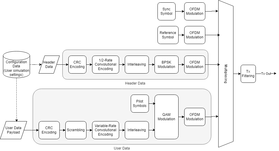
The data symbols comprise a single user populating a single transport block of data transmitted once per frame. The crcGenerate function computes the CRC for the transport block payload and appends it to the payload. The data is additively scrambled using a comm.PNSequence object to distribute the data power evenly across the transmission spectrum. Interleaving is done with the reshape function to resist burst errors caused by deep fades. Convolutional encoding adds redundant bits for forward error correction and is done with the convenc function. Puncturing of the data increases data throughput by reducing the number of redundant bits. The transport block is modulated using the qammod function and is ready for transmission in an OFDM frame. All signals are OFDM-modulated using the ofdmmod function. The signal is filtered to reduce out-of-band emissions using dsp.FIRFilter, with coefficients generated using the firpmord and firpm filter design functions.
        % Transmit data
        [txOut,txGrid,txDiagnostics] = helperOFDMTx(txParam,sysParam,txObj);
Apply Channel and Hardware Impairments
Introduce impairments to corrupt the transmitted signal, including fading, additive white Gaussian noise (AWGN), and carrier frequency offset. The impulse response of the channel is optionally shown to visualize potential inter-symbol interference leaking out of the cyclic prefix region of the OFDM symbol.
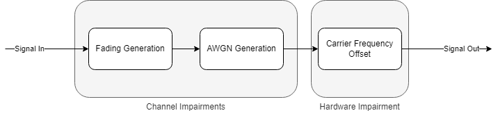
Fading
A comm.RayleighChannel object is used to apply Rayleigh fading to the transmitted output. Using an object allows for channel statistics to be retained internally between calls to the object. Because the Doppler frequency is a function of transmission frequency, the normalized Doppler parameter is used to convey the Doppler frequency and more easily show the impact of mobile speed independent of the carrier frequency.
Additive Noise
The awgn function is used to apply AWGN to the faded signal. The input power into the awgn function is calculated as a function of per-subcarrier constellation power and number of occupied subcarriers. This input power is passed to the awgn function, along with the target SNR, to get the desired signal SNR.
Carrier Frequency Offset
Finally, the frequency offset is applied within the channel block. Use the comm.PhaseFrequencyOffset function to rotate the time-domain signal by the desired frequency.
        % Process one frame of samples through channel
        chanOut = helperOFDMChannel(txOut,chanParam,sysParam);
Channel Visualization
Use the spectrumAnalyzer function to visualize the received spectrum after fading and noise are added to the transmitted signal. As the simulation runs, you can see how the received signal constellation is negatively affected by the spectral nulls caused by multipath fading.
        if userParam.enableScopes
            sa(txOut,chanOut);
        end

Receiver Processing
The receiver reverses the transmitter processing. It also must detect and correct distortions caused by asynchronous timing, frequency offset, noise, time-varying fading, frequency-selective fading, and phase jitter.
The signal is lowpass filtered to remove out-of-band energy that could introduce noise. At the start of the receiver simulation, sync signal detection is performed by time-domain correlation and thresholding to determine the start of the frame. Until the sync symbol is detected, the receiver is not "camped" to any base station.
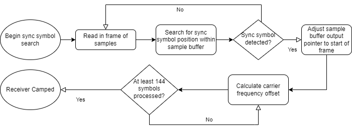
Following successful sync detection, 144 symbols are used by the automatic frequency correction (AFC) to estimate the frequency offset by detecting the phase shift between the cyclic prefix (a copy of the end of the symbol's samples that is transmitted at the beginning of an OFDM symbol) and the end of the symbol. Six symbols are used to obtain one frequency offset estimate, and the last 24 estimates are averaged to obtain the final filtered CFO estimate. Combined with knowledge of the duration of an OFDM symbol, the frequency offset can be estimated using inner product calculation. The frequency offset is then corrected with a numerically controlled oscillator using the comm.PhaseFrequencyOffset object. Once the signal is stable with respect to the timing offset and frequency offset, the receiver is considered camped and connected, and a complete frame is demodulated into OFDM subcarriers using ofdmdemod.
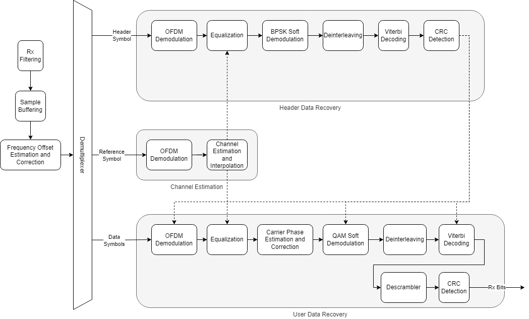
To combat time-varying fading, two reference symbols from adjacent frames are used to estimate the channel at different points in time, and then the channel estimates in between the two reference symbols are linearly interpolated to provide the channel estimates for the header and data symbols. The symbols are then equalized using the channel estimates with ofdmEqualize.
The header is extracted and decoded to obtain the data symbol parameters such as FFT length, subcarrier modulation scheme, and code rate. The data symbols are then demodulated according to the header parameters.
The pilots within the data symbols are used to estimate the common phase error (CPE) typically caused by phase jitter in mmWave transmissions. CPE affects all subcarriers equally. The error is derotated to remove the CPE from the data symbols, and the data subcarriers are soft-decoded into log-likelihood ratios (LLRs) using the qamdemod function.
Once the bitstream is available, the bits are deinterleaved before maximum-likelihood decoding is performed using the vitdec function which implements the Viterbi algorithm. The bits are then descrambled, and the crcDetect function computes the CRC and compares it with the appended CRC within the payload for transport block verification.
        % Run the receiver front-end
        rxIn = helperOFDMRxFrontEnd(chanOut,sysParam,rxObj);

        % Run the receiver processing
        [rxDataBits,isConnected,toff,rxDiagnostics] = helperOFDMRx(rxIn,sysParam,rxObj);
        sysParam.timingAdvance = toff;

        % Collect bit and frame error statistics
        if isConnected
            % Continuously update the bit error rate using the |comm.ErrorRate|
            % system object
            BER = errorRate(...
                sysParam.txDataBits(end-(2*sysParam.trBlkSize)+(1:sysParam.trBlkSize)), ...
                rxDataBits);
        end
Receiver Performance Visualization
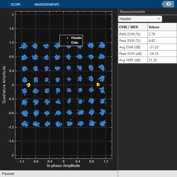
Use the comm.ConstellationDiagram object to display the header constellation and data constellation in one plot. By varying the channel impairments, you can visualize the noise after receiver impairment compensation for all subcarriers superimposed on the plot. EVM and MER can be measured with respect to the reference constellation for each data modulation.
        if isConnected && userParam.enableScopes
            constDiag(complex(rxDiagnostics.rxConstellationHeader(:)), ...
                      complex(rxDiagnostics.rxConstellationData(:)));
        end
    end % frame loop
Sync symbol found.
Estimating carrier frequency offset .............
Receiver camped.
....................................................................
.....................
Sync symbol found.
Estimating carrier frequency offset .............
Receiver camped.
....................................................................
.....................
Sync symbol found.
Estimating carrier frequency offset .............
Receiver camped.
....................................................................
.....................
Clear Simulation and Compute Statistics
Following frame processing, clear out state information stored in persistent variables with the clear command. Accumulated bit error rate and frame error rate statistics are calculated and displayed at the simulated SNR. The simulation loads the next SNR and executes another run.
    % Clear out the |persistent| variables for the sync detection flag and
    % camped flag
    clear helperOFDMRx;
    clear helperOFDMRxSearch;

    % Compute data diagnostics
    if isConnected
        FER = sum(rxDiagnostics.dataCRCErrorFlag) / length(rxDiagnostics.dataCRCErrorFlag);
        fprintf('Simulation completed at %d SNR: BER = %d, FER = %d\n',SNRdB(simLoopIdx),BER(1),FER);
        BERResults(simLoopIdx) = BER(1);
    else
        fprintf('Simulation completed at %d SNR: Base station not detected.\n',SNRdB(simLoopIdx));
        fprintf('\n');
        BERResults(simLoopIdx) = 0.5; % default to high BER for plotting purposes
    end

    % Release object to reconfigure for the next simulation run
    release(errorRate);

% SNR loop end
end
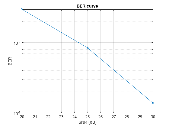
Simulation completed at 20 SNR: BER = 2.964455e-02, FER = 5.056180e-01
Simulation completed at 25 SNR: BER = 8.443698e-03, FER = 2.921348e-01
Simulation completed at 30 SNR: BER = 1.385706e-03, FER = 2.808989e-01
Diagnostics
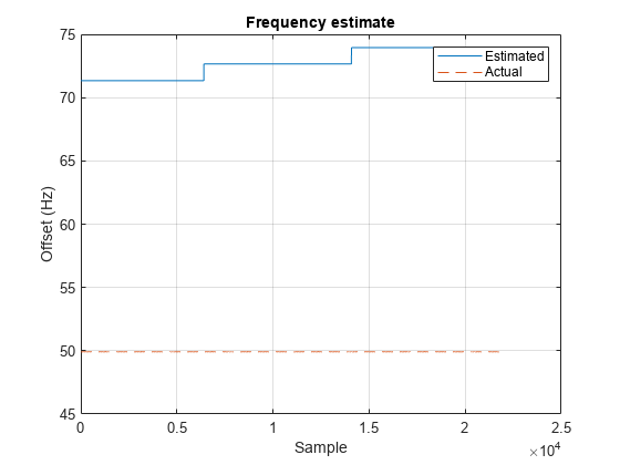
A diagnostic structure captures various parameters for analysis during the simulation. Receiver performance can be recorded and plotted, such as the last frame's frequency offset tracking and channel estimation tracking. Error metrics like BER and FER/BLER can also be calculated and displayed.
% Plot the transmission grid
helperOFDMPlotResourceGrid(txGrid,sysParam);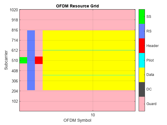
% Plot the frequency offset estimator output
figure;
numFreqOffset = length(rxDiagnostics.estCFO);
numSampPerFreqOffset = (sysParam.FFTLen + sysParam.CPLen) * 6;
numSampFirstFreqOffset = length(rxIn) - (numFreqOffset-1)*numSampPerFreqOffset;
cfoSamples = [numSampFirstFreqOffset; repmat(numSampPerFreqOffset,numFreqOffset-1,1)];
cfoSamples = cumsum(cfoSamples);
cfoSamples = repelem(cfoSamples,2);
cfoSamples = [1; cfoSamples(1:end-1)];
cfoEst = [rxDiagnostics.estCFO, rxDiagnostics.estCFO].';
cfoEst = cfoEst(:)*sysParam.scs;
plot(cfoSamples, cfoEst);
hold on;
plot(foff*fsamp*ones(length(rxIn),1)/1e6,'--');
title('Frequency estimate');
xlabel('Sample');
ylabel('Offset (Hz)');
grid on;
legend('Estimated','Actual');
% Plot the channel estimate for one subcarrier
figure;
plot(real(rxDiagnostics.estChannel(3,:)));
hold on;
plot(imag(rxDiagnostics.estChannel(3,:)));
title('Channel estimate, subcarrier 3');
xlabel('Symbol');
ylabel('Magnitude');
grid on;
legend('Real','Imag');

% Plot a BER curve if more than one SNR was specified
if length(SNRdB) > 1
    figure;
    semilogy(SNRdB,BERResults+eps,'-*'); % add eps if no errors found
    title('BER curve');
    xlabel('SNR (dB)');
    ylabel('BER');
    grid on;
end
Summary
This example utilizes several MATLAB System objects and functions to perform DSP and digital communications operations common within an OFDM transmission system. Various scopes and plots help visualize the signal in both time and frequency domains to evaluate receiver performance.
Appendix
The following helper functions are used in this example:
Setup:
helperOFDMTxInit.m
helperOFDMRxInit.m
helperOFDMSetParameters.m
Common tx/rx helpers:
helperOFDMGetTables.m
helperOFDMFrontEndFilter.m
Transmitter:
helperOFDMTx.m
Channel:
helperOFDMChannel.m
Receiver:
helperOFDMRx.m
helperOFDMRxFrontEnd.m
helperOFDMRxSearch.m
helperOFDMChannelEstimation.m
helperOFDMFrequencyOffset.m
Visualization:
helperOFDMPlotResourceGrid.m
The following helper functions can be modified to generate custom signals:
helperOFDMPilotSignal.m
helperOFDMRefSignal.m
helperOFDMSyncSignal.m