OSTBC Transmission with Antenna Coupling

This example uses:

This example shows how the antenna mutual coupling affects the performance of an orthogonal space-time block code (OSTBC) transmission over a multiple-input multiple-output (MIMO) channel. The transmitter and receiver have two dipole antenna elements each. The BER vs. SNR curves are plotted under different correlation and coupling scenarios. To run this example, you need Antenna Toolbox™.

System Parameters

A QPSK modulated Alamouti OSTBC is simulated over a 2x2 quasi-static frequency-flat Rayleigh channel [ 1 ]. The system operates at 2.4 GHz. The SNR range to be simulated is 0 to 10 dB.

fc = 2.4e9;         % Center frequency
Nt = 2;             % Number of Tx antennas
Nr = 2;             % Number of Rx antennas
blkLen = 2;         % Alamouti code block length
snr = 0:10;         % SNR range
maxNumErrs = 3e2;   % Maximum number of errors
maxNumBits = 5e4;   % Maximum number of bits

Create objects to perform Alamouti encoding and combining, AWGN channel as well as BER calculation.

alamoutiEnc = comm.OSTBCEncoder( ...
    'NumTransmitAntennas', Nt);
alamoutiDec = comm.OSTBCCombiner( ...
    'NumTransmitAntennas', Nt, ...
    'NumReceiveAntennas',  Nr);
awgnChanNC = comm.AWGNChannel( ... % For no coupling case
    'NoiseMethod', 'Signal to noise ratio (SNR)',...
    'SignalPower', 1);
berCalcNC = comm.ErrorRate;       % For no coupling case

% Clone objects for mutual coupling case 
awgnChanMC = clone(awgnChanNC); 
berCalcMC  = clone(berCalcNC);

Antenna Arrays and Coupling Matrices

A two-element resonant dipole array is used at both transmit (Tx) and receive (Rx) side. At Tx, the dipoles are spaced a half-wavelength apart. At Rx, the spacing is a tenth of a wavelength.

txSpacing = 0.5;
rxSpacing = 0.1;
lambda = physconst('lightspeed')/fc;
antElement = dipole( ...
    'Length', lambda/2, ...
    'Width',  lambda/100);
txArray = linearArray( ...
    'Element',        antElement,...
    'NumElements',    Nt,...
    'ElementSpacing', txSpacing*lambda);
rxArray = linearArray( ...
    'Element',        antElement,...
    'NumElements',    Nr,...
    'ElementSpacing', rxSpacing*lambda);

The coupling matrix is calculated based on a circuit model of the array as per [ 2 ]. The s-parameter calculation is performed for the transmit and receive arrays and from this the impedance matrix representation of the array is derived.

txMCMtx = helperCalculateCouplingMatrix(txArray, fc, [1 Nt]);
rxMCMtx = helperCalculateCouplingMatrix(rxArray, fc, [1 Nr]);

Spatial Correlation Matrices

The transmit and receive spatial correlation matrices capture the propagation environment of the channel. Without coupling, it is assumed that the two elements at Tx are uncorrelated and the two elements at Rx have high correlation. The combined/overall correlation matrix for the whole channel is their Kronecker product.

txCorrMtx = eye(2);
rxCorrMtx = [1 0.9; 0.9 1];
combCorrMtx = kron(txCorrMtx, rxCorrMtx);

With coupling, we use the approach in [ 3 ] to modify the Tx and Rx correlation matrices by pre and post-multiplying them by the corresponding coupling matrices. This is valid under the assumption that the correlation and coupling can be modeled independently.

txMCCorrMtx = txMCMtx * txCorrMtx * txMCMtx';
rxMCCorrMtx = rxMCMtx * rxCorrMtx * rxMCMtx';

The combined spatial correlation with coupling is kron(txMCCorr, rxMCCorr). Alternatively, we can treat the Tx/Rx coupling matrix as being "absorbed" into the Tx/Rx correlation matrix and derive the combined correlation matrix as follows:

txSqrtCorrMtx = txMCMtx * sqrtm(txCorrMtx);
rxSqrtCorrMtx = rxMCMtx * sqrtm(rxCorrMtx);
combMCCorrMtx = kron(txSqrtCorrMtx, rxSqrtCorrMtx);
combMCCorrMtx = combMCCorrMtx * combMCCorrMtx';

MIMO Channel Modeling

Create two comm.MIMOChannel objects to simulate the 2x2 MIMO channels with and without coupling. The combined spatial correlation matrix is assigned in each case. The MaximumDopplerShift property of the objects is set to 0 to model a quasi-static channel.

mimoChanNC = comm.MIMOChannel( ...  % For no coupling case 
    'MaximumDopplerShift',             0, ...
    'SpatialCorrelationSpecification', 'Combined', ...
    'SpatialCorrelationMatrix',        combCorrMtx,...
    'PathGainsOutputPort',             true);

% Clone objects for mutual coupling case 
mimoChanMC = clone(mimoChanNC);
mimoChanMC.SpatialCorrelationMatrix = combMCCorrMtx;

Simulations

Simulate the QPSK modulated Alamouti code for each SNR value with and without antenna coupling. One Alamouti code is simulated through the MIMO channel in each iteration. To model a quasi-static channel, we reset the comm.MIMOChannel object to obtain a new set of channel gains for each code transmission (iteration).

% Set up a figure to visualize BER results
h1 = figure; grid on; hold on;
ax = gca;
ax.YScale = 'log';
xlim([snr(1), snr(end)]); ylim([1e-3 1]);
xlabel('SNR (dB)'); ylabel('BER'); 
h1.NumberTitle = 'off';
h1.Name = 'Orthogonal Space-Time Block Coding';
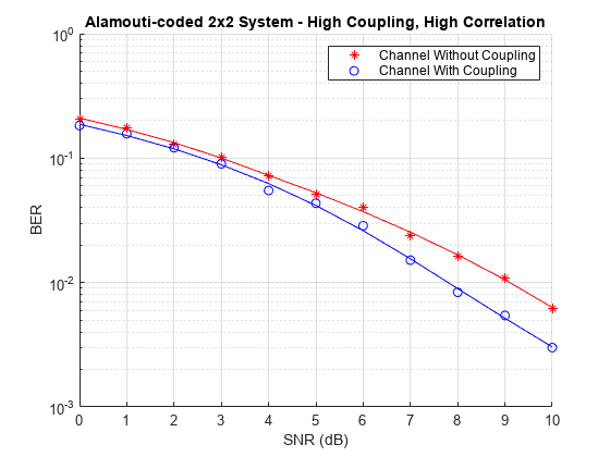
title('Alamouti-coded 2x2 System - High Coupling, High Correlation');

s = rng(108);  % For repeatability
[berNC, berMC] = deal(zeros(3,length(snr)));

% Loop over SNR values
for idx = 1:length(snr)
    awgnChanNC.SNR = snr(idx); 
    awgnChanMC.SNR = snr(idx); 
    reset(berCalcNC); 
    reset(berCalcMC);    
    
    while min(berNC(2,idx),berMC(2,idx)) <= maxNumErrs && (berNC(3,idx) <= maxNumBits)    
        % Generate random data
        txData = randi([0 3],blkLen,1);
        
        % Perform QPSK modulation and Alamouti encoding
        txSig = alamoutiEnc(pskmod(txData,4,pi/4)); 
        
        % Pass through MIMO channel
        reset(mimoChanNC); reset(mimoChanMC);
        [chanOutNC, estChanNC] = mimoChanNC(txSig);
        [chanOutMC, estChanMC] = mimoChanMC(txSig);
        
        % Add AWGN
        rxSigNC = awgnChanNC(chanOutNC);
        rxSigMC = awgnChanMC(chanOutMC);
        
        % Perform Alamouti decoding with known channel state information
        decSigNC = alamoutiDec(rxSigNC,squeeze(estChanNC));
        decSigMC = alamoutiDec(rxSigMC,squeeze(estChanMC));
                        
        % Perform QPSK demodulation 
        rxDataNC = pskdemod(decSigNC,4,pi/4);
        rxDataMC = pskdemod(decSigMC,4,pi/4);
        
        % Update BER
        berNC(:, idx) = berCalcNC(txData,rxDataNC);
        berMC(:, idx) = berCalcMC(txData,rxDataMC);
    end 

    % Plot results
    semilogy(snr(1:idx),berNC(1,1:idx),'r*');
    semilogy(snr(1:idx),berMC(1,1:idx),'bo');
    legend({'Channel Without Coupling','Channel With Coupling'});
    drawnow;
end

% Perform curve fitting
fitBERNC = berfit(snr,berNC(1,:));
fitBERMC = berfit(snr,berMC(1,:));
semilogy(snr,fitBERNC,'r',snr,fitBERMC,'b');
legend({'Channel Without Coupling','Channel With Coupling'});

Figure Orthogonal Space-Time Block Coding contains an axes object. The axes object with title Alamouti-coded 2x2 System - High Coupling, High Correlation, xlabel SNR (dB), ylabel BER contains 24 objects of type line. One or more of the lines displays its values using only markers These objects represent Channel Without Coupling, Channel With Coupling.

rng(s); % Restore RNG

Further Exploration

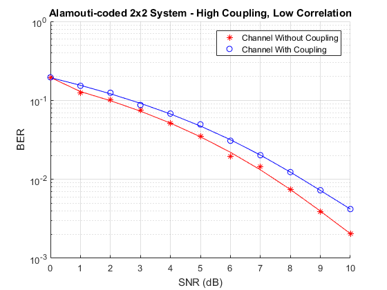
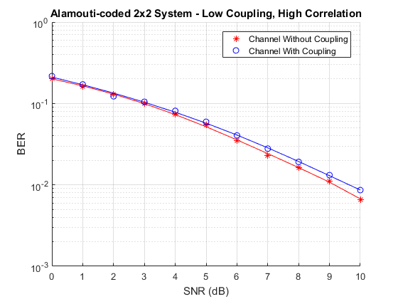
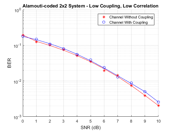
The effect of correlation and mutual coupling on the BER performance can be further studied by modifying the correlation coefficient and/or by changing the spacing between the elements. The smaller the spacing is, the higher the coupling is. Similar to what has been done above for high correlation (0.9) and high coupling (spacing = $0.1 λ$ ) at Rx, we now show the BER vs. SNR results for low correlation (0.1) and/or low coupling (spacing = $0.5 λ$ ).

High Coupling (spacing = $0.1 λ$ ), Low Correlation (0.1)

Low Coupling (spacing = $0.5 λ$ ), High Correlation (0.9)

Low Coupling (spacing = $0.5 λ$ ), Low Correlation (0.1)

Conclusion

The simulation results are similar to those reported in [ 1 ]. A spacing of $0.5 λ$ has a negligible impact on BER under both high and low correlation conditions. For the case with high coupling, i.e., $0.1 λ$ element spacing, the results indicate that depending on the correlation conditions, the BER could be either higher or lower than if coupling were not considered.

Appendix

This example uses the following helper functions:

helperCalculateCouplingMatrix.m

References

1 - A. A. Abouda, H. M. El-Sallabi, and S. G. Haggman, "Effect of Mutual Coupling on BER Performance of Alamouti Scheme," IEEE International Symposium on Antennas and Propagation, July 2006.

2 - I. J. Gupta and A. A. Ksienski, "Effect of mutual coupling on the performance of adaptive arrays," IEEE Trans. on Antennas and Propagation, vol. 31, no. 5, pp. 785-791, 1989.

3 - Y. Wu, J. P. Linnartz, J. W. M. Bergmans, and S. Attallah, "Effects of Antenna Mutual Coupling on the Performance of MIMO Systems," Proc. 29th Symposium on Information Theory in the Benelux, May 2008.