Angular Rate Control in the HL-20 Autopilot

Control Architecture

Open the HL-20 model with its flight control system.

open_system('csthl20_control')

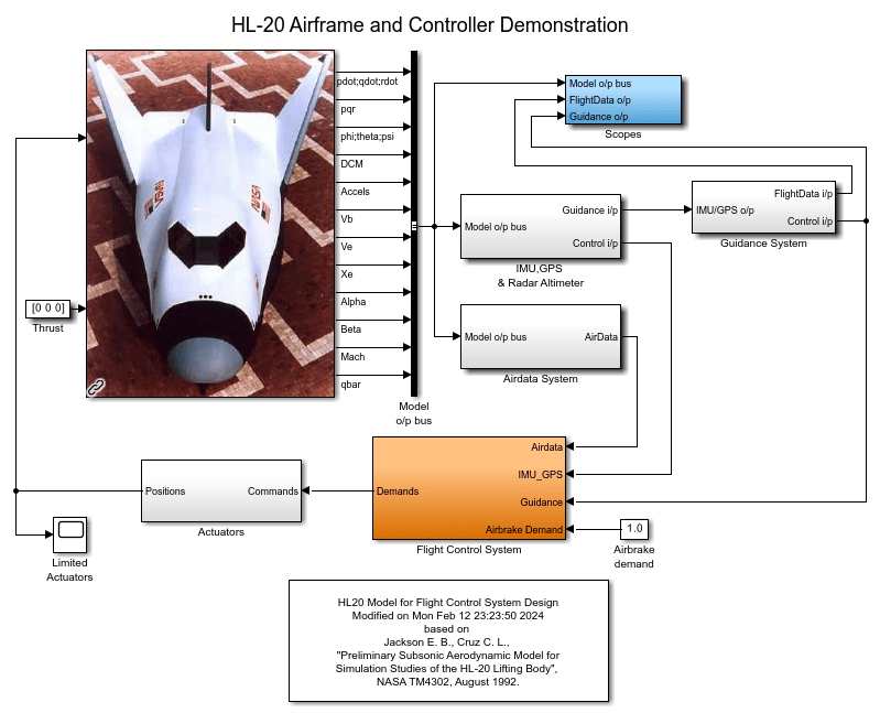
This 6-DOF model is adapted from NASA HL-20 Lifting Body Airframe (Aerospace Blockset). The model is configured to simulate the final approach to the landing site. The "Guidance System" generates the glideslope trajectory and corresponding roll, angle of attack (alpha), and sideslip angle (beta) commands. The "Flight Control System" is tasked with adjusting the control surfaces to track these commands. The "Controller" block inside the "Flight Control System" is a variant subsystem with different autopilot configurations.

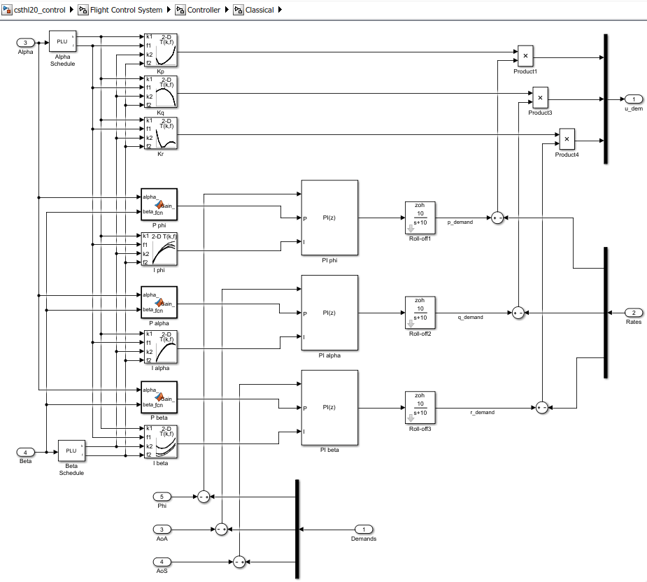
The "Baseline" and "Classical" controllers use a classic cascaded-loop architecture with three inner P-only loops to control the angular rates p,q,r, and three outer PI loops to control the angular positions phi,alpha,beta. The six proportional gains and three integral gains are all scheduled as a function of alpha and beta. The "Baseline" variant contains the baseline design featured in NASA HL-20 Lifting Body Airframe (Aerospace Blockset). Parts 2 and 3 of this series use the "Classical" variant to walk through the tuning process. The active variant is controlled by the workspace variable CTYPE. Set its value to 2 to activate the "Classical" variant of the controller.

% Select "Classical" variant of controller
CTYPE = 2;

% call model update to make sure only active variant signals are analyzed during linearization
set_param('csthl20_control', 'SimulationCommand', 'update');

Note that this variant uses a mix of lookup tables and MATLAB Function blocks to schedule the autopilot gains.

Setup for Controller Tuning

In Part 1 of this series (Trimming and Linearization of the HL-20 Airframe), we obtained linearized models of the "HL20 Airframe" and "Controls Selector" blocks for 40 different aircraft orientations (40 different pairs of (alpha,beta) values). Load these arrays of linearized models.

load csthl20_TrimData G7 CS

size(G7)

8x5 array of state-space models.
Each model has 34 outputs, 9 inputs, and 7 states.

size(CS)

8x5 array of state-space models.
Each model has 6 outputs, 5 inputs, and 0 states.

The slTuner interface is a convenient way to obtain linearized models of "csthl20_control" that are suitable for control system design and analysis. Through this interface you can designate the signals and points of interest in the model and specify which blocks you want to tune.

ST0 = slTuner('csthl20_control');
ST0.Ts = 0;   % ask for continuous-time linearizations

Here the points of interest include the angular and rate demands, the corresponding responses, and the deflections da,de,dr.

AP = {'da;de;dr'
   'HL20 Airframe/pqr'
   'Alpha_deg'
   'Beta_deg'
   'Phi_deg'
   'Controller/Classical/Demands'  % angular demands
   'p_demand'
   'q_demand'
   'r_demand'};
ST0.addPoint(AP)

Since we already obtained linearized models of the "HL20 Airframe" and "Controls Selector" blocks as a function of (alpha,beta), the simplest way to linearize the entire model "csthl20_control" is to replace each nonlinear component by a family of linear models. This is called "block substitution" and is often the most effective way to linearize complex models at multiple operating conditions.

% Replace "HL20 Airframe" block by 8-by-5 array of linearized models G7
BlockSub1 = struct('Name','csthl20_control/HL20 Airframe','Value',G7);

% Replace "Controls Selector" by CS
BlockSub2 = struct('Name','csthl20_control/Flight Control System/Controls Selector','Value',CS);

% Replace "Actuators" by direct feedthrough (ignore saturations and second-order actuator dynamics)
BlockSub3 = struct('Name','csthl20_control/Actuators','Value',eye(6));

ST0.BlockSubstitutions = [BlockSub1 ; BlockSub2 ; BlockSub3];

You are now ready for the control design part.

Closing the Inner Loops

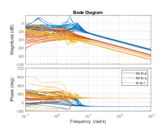
Begin with the three inner loops controlling the angular rates p,q,r. To get oriented, plot the open-loop transfer function from deflections (da,de,dr) to angular rates (p,q,r). With the slTuner interface, you can query the model for any transfer function of interest.

% NOTE: The second 'da;de;dr' opens all feedback loops at the plant input
Gpqr = getIOTransfer(ST0,'da;de;dr','pqr','da;de;dr');

bode(Gpqr(1,1),Gpqr(2,2),Gpqr(3,3),{1e-1,1e3}), grid
legend('da to p','de to q','dr to r')

This Bode plot suggests that the diagonal terms behave as integrators (up to the sign) beyond 5 rad/s. This justifies using proportional-only control. Consistent with the baseline design, set the target bandwidth for the p,q,r loops to 30, 22.5, and 37.5 rad/s, respectively. The gains Kp, Kq, Kr for each (alpha,beta) value are readily obtained from the plant frequency response at these frequencies, and the phase plots indicate that Kp should be positive (negative feedback) and Kq, Kr should be negative (positive feedback).

% Compute Kp,Kq,Kr for each (alpha,beta) condition. Resulting arrays
% have size [1 1 8 5]
Kp = 1./abs(evalfr(Gpqr(1,1),30i));
Kq = -1./abs(evalfr(Gpqr(2,2),22.5i));
Kr = -1./abs(evalfr(Gpqr(3,3),37.5i));

bode(Gpqr(1,1)*Kp,Gpqr(2,2)*Kq,Gpqr(3,3)*Kr,{1e-1,1e3}), grid
legend('da to p','de to q','dr to r')

To conclude the inner-loop design, push these gain values to the corresponding lookup tables in the Simulink® model and refresh the slTuner object.

MWS = get_param('csthl20_control','ModelWorkspace');
MWS.assignin('Kp',squeeze(Kp))
MWS.assignin('Kq',squeeze(Kq))
MWS.assignin('Kr',squeeze(Kr))

refresh(ST0)

Next you need to tune the outer loops controlling roll, angle of attack, and sideslip angle. Part 3 of this series (Attitude Control in the HL-20 Autopilot - SISO Design) shows how to tune a classic SISO architecture and Part 4 (Attitude Control in the HL-20 Autopilot - MIMO Design) looks into the benefits of a MIMO architecture.